Abstract
The objective of the paper is to simulate the behaviours of mild steel at different strain rates (1-1500s-1) under tension and compression by using finite element analysis code in ANSYS. Numerical simulation are done using Cowper-Symonds (C-S) and Johnson-Cook (J-C) material models to represent the flow stresses of mild steel. The simulated results have good agreement with the predicted results of the above material models.
Highlights
- Numerical simulation on dynamic behaviour of mild steel under tension and compression.
- Material models such as Johnson-Cook and Cowper-Symonds models.
- Strain hardening and material sensitivity at low, medium and high strain rates.
1. Introduction
Numerical simulation of a problem is always appreciated. The assessment of the simulated results depends on the capabilities of mathematical models of the problem. Sometimes, it is very difficult to perform experiments due to unavailability of required equipment. Costlier experiments are also not recommended. In this case, the existing models play important roles for solving problems. There are many authors (Doner et al. [1], Kaufhold et al. [2], Wang et al. [3], Nayyeri et al. [4]) who have worked on modelling and simulation on different metallic materials. This paper is based on the numerical simulation of the experimental work presented by Singh et al. [5] in which obtained material parameters of C-S model [6] and J-C model [7] are used to simulate the problem in ANSYS. It is found that the simulated results have good agreement with the analytical (predicted) results of the models and the experimental results.
2. Methodology
The virtual 3-D models (Fig. 1) of specimens for tensile and compressive tests are created in CATIA V5R18. Information regarding the material and the constitutive models (C-S and J-C) are specified in engineering data and the geometry of the physical model is defined in ANSYS. Then the 3-D CATIA models are imported to ANSYS workbench in .igs file format for analysis. For Cowper-Symonds model, it is required to mention five parameters such that , , and two material constants ( and ) whereas, for Johnson-Cook model to be used, it is required to mention seven parameters such as , , , , (= 1), melting temperature (1510 °C) and reference strain rate (0.001 s-1).
Fig. 13-D models of specimens under a) tension and b) compression
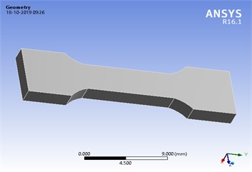
a)
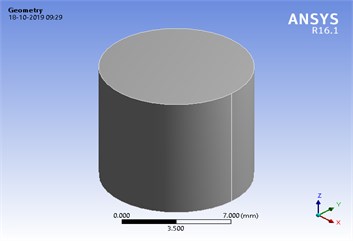
b)
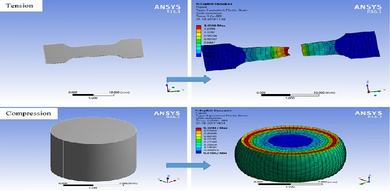
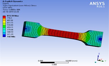
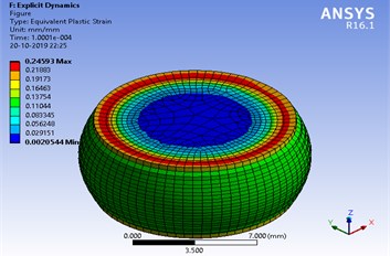
Here, medium size is considered for meshing and then simulation is done in ANSYS. The simulated specimens are shown in Fig. 2. In tension, number of elements and nodes are 1392 and 2015 respectively. In compression, number of elements and nodes are 12528 and 14000 respectively. The type of element is hexahedron with eight nodes in both tension and compression. For analysis in ANSYS, velocity is taken as input parameter. In both tension and compression, the models are fixed at one end and velocity corresponding to different strain rate is applied at another end. The required output parameters are selected in solution tab such as deformation, stress, strain etc. After simulation, the deformed geometrical shapes of specimens are as shown in Fig. 3.
Fig. 2Medium meshed geometrical model for tension and compression
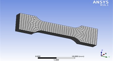
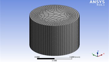
Fig. 3Deformation in specimens for tension (750 s-1) and compression (1300 s-1)
3. Finite element analysis simulation using ANSYS
The experimental work presented by Singh et al. [5] is simulated using ANSYS 16.1 at low, medium and high strain rates (1-1500 s-1) under tension and compression. Here, the thermal softening parameter 1 is taken. The numerical simulation performed on 2.30 GHz processor computer in different time duration for various strain rates under tension and compression. The time scale for each process is chosen such that it covers up the flow stresses as determined by Singh et al. [5]. It is observed the computation time for performing analysis decreases with increasing strain rate. True yield stresses (at 0.2 % strain) corresponding to different strain rates as obtained from simulation are compared with the predicted values of C-S and J-C models in Table 1 and Table 2 respectively whereas, the flow stresses are compared in Figs. 4-6.
Fig. 4Comparison between the simulated results in ANSYS and the predicted results by Cowper-Symonds model at different strain rates under tension and compression
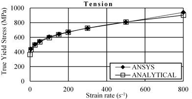
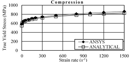
Table 1True yield stress corresponding to different strain rates using Cowper-Symonds model
Strain rate (s-1) | Tension | Compression | ||
ANSYS | Analytical | ANSYS | Analytical | |
1 | 405 | 398.8 | 585 | 580.31 |
5 | 439.88 | 431.8 | 597.85 | 600.66 |
25 | 504.34 | 495.22 | 644.33 | 633.07 |
50 | 545.84 | 538.19 | 665.7 | 652.4 |
100 | 606.29 | 595.1 | 681.26 | 676.01 |
150 | 643.83 | 636.62 | 708 | 692.19 |
200 | 673.84 | 670.51 | 722 | 704.88 |
300 | 723.77 | 725.51 | 744 | 724.65 |
500 | 807.62 | 809.02 | 776 | 753.09 |
800 | 941.9 | 902.76 | 810 | 783.25 |
1000 | 1029.9 | 953.93 | 828 | 799.06 |
1200 | 1085.4 | 999.32 | 843 | 812.77 |
1500 | 1140 | 1059.63 | 864 | 830.55 |
Table 2True yield stress corresponding to different strain rates using Johnson-Cook model
Tension | Compression | ||||
Strain rate (s-1) | ANSYS | Analytical | Strain rate (s-1) | ANSYS | Analytical |
1 | - | 405.58 | 1 | 617.35 | 619 |
5 | 416 | 418.015 | 125 | 724 | 718.065 |
25 | 452 | 450.757 | 550 | 770 | 765.867 |
250 | 500 | 493.295 | 800 | 793 | 790.216 |
500 | 506 | 500.85 | 1100 | 800 | 796.84 |
750 | 510 | 507.624 | 1300 | 818 | 808.551 |
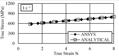
Fig. 5Comparison between the simulated results in ANSYS and the predicted results of Johnson-Cook model at different strain rates under tension
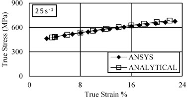
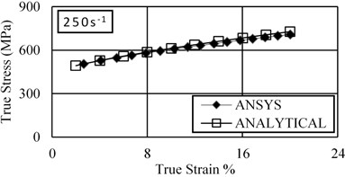
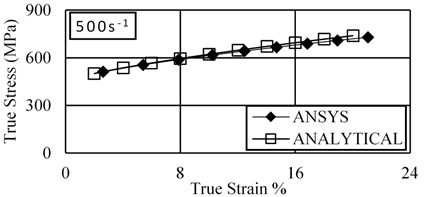
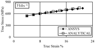
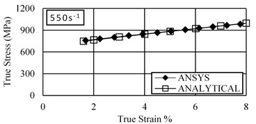
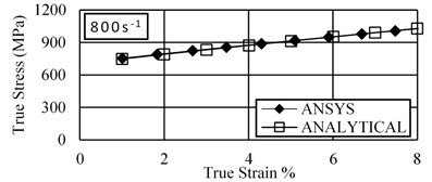
Fig. 6Comparison between simulated results and predicted results by Johnson-Cook model at different strain rates under compression
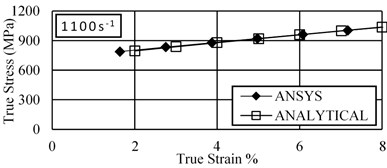
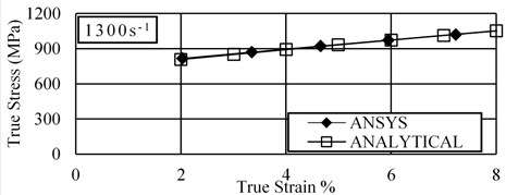
4. Conclusions
Flow behaviours of mild steel are discussed through the numerical simulation in ANSYS. Strain hardening and material sensitivity are found similar as obtained experimentally by Singh et al. [5]. Results achieved from numerical simulations have good agreement with the predicted results by C-S and J-C models under tension and compression.
References
-
Doner S., Nayak S., Senol K., Shukla A., Krishnan N. M. A., Yilmazcoban I. K., Das S. Dynamic compressive behavior of metallic particulate-reinforced cementitious composites: SHPB experiments and numerical simulations. Construction and Building Materials, Vol. 22, 2019, p. 116668.
-
Kaufhold C., Pöhl F., Mottyll S., Skoda R., Theisen W. Numerical simulation of the deformation behavior of metallic materials under cavitation induced load in the incubation period. Wear, Vols. 376-377, 2017, p. 1138-1146.
-
Wang Z., Wang X., Shi C., Li Z., Zhou W. Mechanical behaviors of square metallic tube reinforced with rivets-Experiment and simulation. International Journal of Mechanical Sciences, Vol. 163, 2019, p. 105118.
-
Nayyeri M. J., Mirbagheri S. M. H., Fatmehsari D. H. Compressive behavior of tailor-made metallic foams (TMFs): numerical simulation and statistical modeling. Materials and Design, Vol. 84, 2015, p. 223-230.
-
Singh N. K., Cadoni E., Singha M. K., Gupta N. K. Dynamic tensile and compressive behaviors of mild steel at wide range of strain rates. Journal of Engineering Mechanics, Vol. 139, Issue 9, 2013, p. 1197-1206.
-
Cowper G. R., Symonds P. S. Strain Hardening and Strain Rate Effects in the Impact Loading of Cantilever Beams. Report No. 28, Brown University, 1957.
-
Johnson G. R., Cook W. H. A. A constitutive model and data for metals subjected to large strains, high strain rates and high temperatures. Proceedings of the 7th International Symposium on Ballistics, Florida, 1983, p. 541-547.
Cited by
About this article

