The mathematical model of the improved system of the seat with adjustable pressure profile

Tran Xuan, Tien; Phu, Dong Nguyen

doi:10.21595/mme.2019.21211

Mathematical Models in Engineering

Browse Journal

Submit article

Published: 30 June 2020

Check for updates

The mathematical model of the improved system of the seat with adjustable pressure profile

Tien Tran Xuan¹

Dong Nguyen Phu²

¹Department of Mechatronics, Faculty of Mechanical Engineering, Hung Yen University of Technology and Education, Hung Yen, Vietnam

²Department of Vehicles and Engines, Faculty of Mechanical Engineering, Technical University of Liberec, Liberec, Czech Republic

Corresponding Author:

Tien Tran Xuan

Cite the article Download PDF

Abstract

Following a patented solution, a seat which is possible to change its stiffness was created. The seat contains an actively controlled pneumatic spring element (the PSE). For the requirement of working faster and more precisely, an improvement was applied. This article deals with derivation of mathematical model of the improved PSE system used for subsequent analysis. The model is considered as a mixed model which is a combination of single-discipline subsystems as mechanical, electrical, fluid and control ones. The simulations are carried out for varied input parameters and both the system parameters and system characteristics are calculated. The results describe the behavior of the improved system in two modes of controller setup: constant pressure and constant stiffness under static and dynamic conditions

1. Introduction

The seat with adjustable pressure profile is shown in Fig. 1(a). A PSE inserted inside the cushion allows changing the stiffness of cushion by a system of pneumatic actuator and a controller [1]. The PSE is inserted inside the car seat cushion (as shown in Fig. 1(b)). The mathematical model of the original system was presented in the article [2]. For the requirement of working faster and more precisely, the improved system is built. The detailed scheme of the system is in Fig. 2.

Fig. 1The seat with a PSE inserted inside

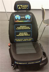
a) The seat in reality

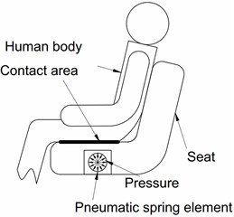
b) A simplified scheme

From the point of view that the PSE affects the human body locally (in contact with buttock), the model is built with the assumption that the mechanical subsystem represents a combination of foam block 100×100×50 mm³ and a PSE (see Fig. 3). An additional latex tube is connected to the PSE (see Fig. 4). It can be considered that the volume change is not caused by the PSE but is caused by the additional latex tube when compressed air is supplied. Therefore, the volume change in case of improved PSE is much larger than in case of the original PSE and the regulation of pressure can be enhanced.

Fig. 2Detailed scheme of the improved system

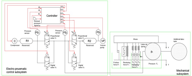
For convenience of modeling, the improved system is divided into two parts: electro-pneumatic control subsystem and mechanical subsystem.

Fig. 3The brick of foam with a PSE inserted inside

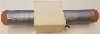
Fig. 4The PSE connected to an additional latex tube

For the distribution of compressed air in and out of the PSE, the system of valves is divided into two pairs. Each pair (input and output) consisting of one proportional valve and one discrete valve. The first pair of input valves ( $V_{1}$ , $V_{3}$ ) is used to distribute the compressed air supplied from the reservoir $R_{1}$ into the PSE, the second pair of output valves ( $V_{2}$ , $V_{4}$ ) is to distribute the air from the PSE to the outlet. A vacuum pump generating output pressure (inside a reservoir $R_{2}$ ) less than 0 kPa is connected to the outlet valves. The proportional valves $V_{1}$ , $V_{2}$ are intended for small airflow in case of small control error (the difference between desired and instant value) which is less than the threshold value set in the control software. The discrete valves $V_{3}$ , $V_{4}$ for faster airflow are opened when the difference between the desired and the instant pressure value is bigger than the threshold value. Sensor PS₁ (SMC PSE540A-R06) measures pressure in the reservoir $R_{1}$ (denoted $p_{c r}$ ) and sensor PS₂ (PSE543A-R06) measures pressure inside the PSE (denoted $p_{s}$ ) and one more sensor PS₃ (PSE543A-R06) is added for measuring vacuum pressure inside the reservoir $R_{2}$ (denoted $p_{v r}$ ). The control software was created in Labview environment. It enables to display the courses of system values in time as desired pressure in PSE, measured unfiltered and filtered pressure in PSE, value of control error, etc. According to [3], the control software is also used for setting of system parameters as upper and lower limit value of pressure in the reservoir, constants of PID controller, selection of working mode (there are 2 modes: constant pressure and constant stiffness). The improved system can work with inlet air pressure up to 250 kPa and vacuum pressure at the output up to –60 kPa. The pressure inside the PSE can be changed in the range [0, 25] kPa.

2. Mathematical model

2.1. Model of the electro-pneumatic control subsystem

The components of this part are proportional and discrete valves, compressor and PID controller.

2.1.1. Model of the valves

The proportional valves denoted $V_{1}$ and $V_{2}$ are of type SMC-PVQ13-6M-08-M5-A. They are characterized by dependence of flow rate $q_{s j}$ ( $j =$ 1, 2) on pressure difference $∆ p$ ( $∆ p = p_{i n l e t} - p_{o u t l e t}$ ) and coil current $i_{j}$ (which is supplied to control the proportional valve $j$ ). The course of these characteristics is taken from the datasheet [3] and it is transformed by means of data-fit algorithm into a two-parametric Eq. (1):

1

q_{s j} = q_{p v} (i_{j}, Δ p) = k_{00} + k_{10} i_{j} Δ p + k_{01} Δ p + k_{20} {i_{j}}^{2}

+ k_{11} i_{j} Δ p + k_{02} Δ p^{2} + k_{30} {i_{j}}^{3} + k_{21} {i_{j}}^{2} Δ p + k_{12} i_{j} Δ p^{2} + k_{03} Δ p^{3},

where: $p_{i n l e t} = p_{c r}$ , $p_{o u t l e t} = p_{s}$ for valve $V_{1}$ and $p_{i n l e t} = p_{s}$ , $p_{o u t l e t} = p_{v r}$ for valve $V_{2}$ .

For the purpose of controlling the system, we define a pressure error e as a difference between desired pressure $p_{d}$ inside the PSE and instant internal pressure $p_{s}$ Eq. (2):

2

e = p_{s} - p_{d} .

Beside that we define a threshold $e_{t}$ which addresses an insensitivity of control system. We have:

3

q_{s 1} = \{\begin{array}{l} q_{p v} (i_{1}, p_{c r} - p_{s}), e < - e_{t}, \\ 0, e \geq - e_{t}, \end{array}

4

q_{s 2} = \{\begin{array}{l} q_{p v} (i_{2}, p_{s} - p_{a t m}), e > e_{t}, \\ 0, e \leq e_{t} . \end{array}

The PID controller is used for control of the coil current which is supplied to proportional valves $V_{1}$ , $V_{2}$ . Using the equation of PID controller the coil current is a function of the pressure error $e$ and it is presented in the form:

5

i_{j} = K_{P} e + K_{I} \int_{0}^{t} e (τ) d τ + K_{D} \frac{d e}{d t},

where: $i_{j} (t)$ is the current supplied for controlling the proportional valve $j$ ( $j =$ 1, 2).

For cases when we need to realize considerably higher flow rates to make system work faster we need to use the pair of discrete valves $V_{3}$ , $V_{4}$ (in the type of SMC-S070B-6A) which increase the flow rate in step-change. According to [4], flow characteristics of the discrete valve include sonic conductance $C_{d v} =$ 0.083 l/(s.bar) and critical pressure ratio $b_{d v} =$ 0.28. The formula for the flow rate calculation of discrete valve is:

6

\frac{p_{d o w n s t r e a m}}{p_{u p s t r e a m}} \leq b_{d v} \to q_{s j} = q_{d v 1} (p_{u p s t r e a m}) = 600 C_{d v} p_{u p s t r e a m} \sqrt{\frac{293}{273 + T}} l / m i n,

in case of choked flow, and:

7

\frac{p_{d o w n s t r e a m}}{p_{u p s t r e a m}} \geq b_{d v} \to q_{s j} = q_{d v 2} (p_{d o w n s t r e a m}, p_{u p s t r e a m}) = 600 C_{d v} p_{u p s t r e a m} \sqrt{1 - {(\frac{\frac{p_{d o w n s t r e a m}}{p_{u p s t r e a m}} - b_{d v}}{1 - b})}^{2}} \sqrt{\frac{293}{273 + T}} l / m i n,

in case of subsonic flow where $j =$ 3, 4.

$p_{u p s t r e a m}$ , $p_{d o w n s t r e a m}$ represents upstream pressure and downstream pressure of the valve respectively. In case of valve $V_{3}$ , $p_{u p s t r e a m} = p_{c r}$ and $p_{d o w n s t r e a m} = p_{s}$ , in case of valve $V_{4}$ , $p_{u p s t r e a m} = p_{s}$ and $p_{d o w n s t r e a m} = p_{a t m}$ , and $T$ is the temperature inside the PSE which is assumed to be constant (297 °K).

The discrete valves $V_{3}$ , $V_{4}$ are used for increasing of airflow when control error is recognized as high which is beyond the sum of the threshold ( $e_{t}$ ) and another parameter (denoted $Δ p_{s}$ ) which is set in the control software and called the value of pressure sensitivity. We have:

8

q_{s 3} = \{\begin{array}{l} q_{d v 1} (p_{c r}), \frac{p_{c r}}{p_{s}} \leq b_{d v}, e < - e_{t} - Δ p_{s}, \\ q_{d v 2} (p_{c r}, p_{s}), \frac{p_{c r}}{p_{s}} \geq b_{d v}, e < - e_{t} - Δ p_{s}, \\ 0, e \geq - e_{t} - Δ p_{s}, \end{array}

9

q_{s 4} = \{\begin{array}{l} q_{d v 1} (p_{s}), \frac{p_{s}}{p_{a t m}} \leq b_{d v}, e > e_{t} + Δ p_{s}, \\ q_{d v 2} (p_{s}), \frac{p_{s}}{p_{a t m}} \geq b_{d v}, e > e_{t} + Δ p_{s}, \\ 0, e \leq e_{t} + Δ p_{s} . \end{array}

2.1.2. Mathematical model of the compressed air supply

The process of transporting air from the compressor to the reservoir and distributing compressed air from the reservoir through inlet valves ( $V_{1}$ and $V_{3}$ ) to the PSE is shown in Fig. 5. The compressor characteristics in time and pressure domain are calculated on the experimental basis. Based on the scheme, the total air flowrate $q_{c r}$ through the reservoir is then given by:

10

q_{c r} = q_{c} - q_{s 1} - q_{s 3},

where: $q_{s 1}$ , $q_{s 3}$ are flow rates of both valves $V_{1}$ , $V_{3}$ , $q_{c}$ is supplied flow rate from the compressor.

Fig. 5The scheme of the process of transmitting compressed air to PSE

When the compressor is working, the flow rate $q_{c}$ can be expressed in form of a linear function of the pressure inside the reservoir $p_{c r}$ :

11

q_{c} = a_{1} (\frac{p_{c r} - p_{a t m}}{b_{1}}) .

The constants $a_{1} =$ 0.062, $b_{1} =$ 275.92 are experimentally determined to correspond to the results in Fig. 6(b).

Pressure $p_{c r}$ is measured by sensor $P S_{1}$ and it is kept in the interval $[p_{c r 1,} p_{c r 2}]$ by the control system. Values $p_{c r 1}$ , $p_{c r 2}$ are set in control software as user-defined system parameters. The compressor is switched on in case $p_{c r} < p_{c r 1}$ (State = ON) and switched off in case of $p_{c r} > p_{c r 2}$ (State = OFF). The “State” is an internal variable that is automatically set by the controller. Normally, the values of $p_{c r 1}$ and $p_{c r 2}$ are set to 190 kPa and 210 kPa respectively. The function describing the flow from the compressor to the reservoir is presented as follows:

12

\{\begin{array}{l} q_{c} = a_{1} (\frac{p_{c r} - p_{a t m}}{b_{1}}), S t a t e = O N, p_{c r} < p_{c r 1}, \\ q_{c} = 0, S t a t e = O F F, p_{c r} > p_{c r 2}, \\ q_{c} = a_{1} (\frac{p_{c r} - p_{a t m}}{b_{1}}), S t a t e = O N, p_{c r 1} < p_{r} < p_{c r 2}, \\ q_{c} = 0, S t a t e = O F F, p_{c r 1} < p_{c r} < p_{c r 2} . \end{array}

Fig. 6The characteristics of the compressor

a) Dependence of pressure of compressed air on time

b) Dependence of flowrate air on pressure

Fig. 7The scheme of the process of releasing compressed air in the improved system

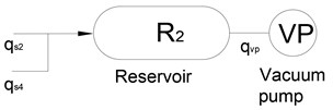
2.1.3. Mathematical model of the vacuum pump

The mathematical model of the vacuum pump can be built similarly to the model of the air compressor because of the same operating principle. The total flow rate through the reservoir is then given by:

13

q_{v r} = - q_{v p} + q_{s 2} + q_{s 4},

where $q_{s 2}$ , $q_{s 4}$ are flow rates of valves $V_{2}$ , $V_{4}$ respectively. In this case $q_{s 2}$ , $q_{s 4}$ is calculated by Eqs. (6) or (7) with $p_{u p s t r e a m} = p_{s}$ and $p_{d o w n s t r e a m} = p_{v r}$ .

When the vacuum pump works the flow rate $q_{v p}$ can be expressed in the form of a linear function of the pressure $p_{r 2}$ inside the reservoir $R_{2}$ :

14

q_{v p} = a_{2} (\frac{p_{v r} - p_{a t m}}{b_{2}}) .

Fig. 8The characteristics of the vacuum pump

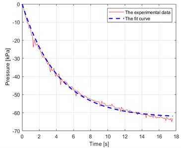
a) Pressure of vacuum pump – time diagram

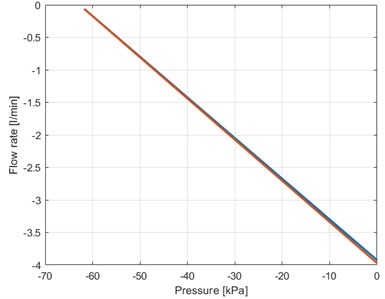
b) Flow rate – pressure diagram

The constants $a_{2} =$ 0.23778, $b_{2} =$ –62.754 are experimentally determined in correspondence with the results in Fig. 8(b).

Pressure $p_{v r}$ is measured by sensor $P S_{3}$ and is kept in the interval $[p_{v r 1,} p_{v r 2}]$ by the control system. Values $p_{v r 1}$ , $p_{v r 2}$ are set in control software as user-defined system parameters. The vacuum pump is switched on in case of $p_{v r} > p_{v r 2}$ (State = ON) and switched off in case of $p_{v r} < p_{v r 1}$ (State = OFF). The “State” is an internal variable that is automatically set by the controller. Normally the values of $p_{v r 1}$ and $p_{v r 2}$ are set to –60 kPa and –40 kPa respectively. The function describing the flow from the reservoir to the vacuum pump is expressed by:

15

\{\begin{array}{l} q_{v p} = a_{2} (\frac{p_{v r} - p_{a t m}}{b_{2}}), S t a t e = O N, p_{v r} > p_{v r 2}, \\ q_{v p} = 0, S t a t e = O F F, p_{r 2} < p_{v r 1}, \\ q_{v p} = a_{2} (\frac{p_{v r} - p_{a t m}}{b_{2}}), S t a t e = O N, p_{v r 1} < p_{v r} < p_{v r 2}, \\ q_{v p} = 0, S t a t e = O F F, p_{v r 1} < p_{v r} < p_{v r 2} . \end{array}

2.2. Model of the mechanical subsystem

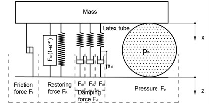
Forces acting on the mass are illustrated in the free-body diagram (see Fig. 9) where $x$ , $\dot{x}$ , $\ddot{x}$ represent the kinematic displacement excitation, velocity excitation and acceleration excitation, ${\vec{F}}_{f o a m}$ , ${\vec{F}}_{p}$ represent the contact forces between the foam block, the latex air spring and the mass sequentially. It is possible to set up the equation of motion of mass $m$ in the form:

16

m g - F_{f o a m} - F_{p} = m \ddot{x} .

For further model derivation, we used this simplified approach.

Fig. 9Free-body diagram

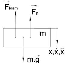
Fig. 10Detailed scheme of the mechanical subsystem.

2.2.1. Model of polyurethane foam

Computational scheme of the rheological model the PU foam block is depicted in Fig. 10. It is the result of research taken from [6]. The concept of this lumped parameter model follows from the phenomenological approach. It comprises nonlinear restoring force $F_{R}$ , damping force $F_{d}$ and frictional force $F_{f}$ in general force response $F_{f o a m}$ . The model definition of PU foam is described in detail as below:

17

F_{f o a m} = F_{f o a m} (x, \dot{x}, x_{d i}, {\dot{x}}_{d i}) = F_{R} (x) + F_{d} (x, \dot{x}, x_{d i}, {\dot{x}}_{d i}) + F_{f} (x, \dot{x}, x_{d i}, {\dot{x}}_{d i}),

18

F_{R} = F_{b} + F_{d p},

19

F_{d} = \sum_{i = 1}^{3} F_{d i},

20

F_{f} = f_{f} F_{R d},

21

F_{b} = F_{b 0} (1 - e^{- c_{b} (x - z)}) F_{b} = F_{b 0} . (1 - e^{- c_{b} (x - z)}),

22

F_{d p} = p_{p} S_{p} [{(\frac{h_{p}}{h_{p} - (x - z)})}^{n_{p}} - {(\frac{h_{p}}{h_{p} + (x - z)})}^{n_{p}}],

23

F_{d i} = F_{d c} (x, x_{d i}) = p_{0 i} S_{0 i} [{(\frac{h_{i}}{h_{i} - (x - x_{d i})})}^{n_{0 i}} - {(\frac{h_{i}}{h_{i} + (x - x_{d i})})}^{n_{0 i}}],

24

F_{f} = f_{f} F_{R d},

25

f_{f} = \frac{2 f_{f 0}}{π} a r c t a n (k_{1} v) + k_{2} {|v|}^{k_{3}} s g n (v) .

The parameter of PU foam model is shown in Table 1.

Table 1The parameter of PU foam model

Force component	Parameter	Physical unit	Value
$F_{b}$	$F_{b 0}$ $c_{b}$	[N] [N/m]	80 600
$F_{d p}$	$S_{p}$ $p_{p}$ $n_{p}$ $h_{p}$	[m²] [Pa] [1] [m]	0.0095 100 6.2 0.06
$F_{d i}$	$S_{0 i}$ $p_{0 i}$ $n_{0 i}$ $h_{i}$ $c_{i}$ $n_{i}$	[m²] [Pa] [1] [m] [-] [1]	$i =$ 1 1.2 100 3 0.05 50 0.2	$i =$ 2 0.03 3.5 0.05 300 0.2	$i =$ 3 0.8 2 0.18 300 0.2
$F_{f}$	$f_{f 0}$ $k_{1}$ $k_{2}$ $k_{3}$	[1] [s/m] [–] [1]	0.05 5000 0.2 1

2.2.2. Model of the combination of the latex air spring and the additional latex tube

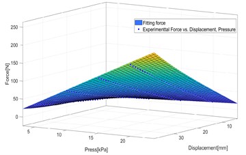
The contact force $F_{p}$ can be considered as a function depending on the deformation ( $x$ - $z$ ) and pressure $p_{s}$ . The change of pressure, deformation and change of contact area is a complex phenomenon, therefore, the dependence of contact force on the deformation and the pressure is determined experimentally. In this way, an experiment was performed on the Instron E3000 machine as shown in Fig. 11. The contact force $F_{p}$ is possible to consider in the form of polynomial function:

26

F_{p} = F_{p} (x, p_{s}) = k_{00} + k_{10} (x - z) + k_{01} (p_{s} - p_{a t m}) + k_{20} {(x - z)}^{2}

+ k_{11} (x - z) (p_{s} - p_{a t m}) + k_{02} {(p_{s} - p_{a t m})}^{2} + k_{30} {(x - z)}^{3}

+ k_{21} {(x - z)}^{2} (p_{s} - p_{a t m}) + k_{12} (x - z) {(p_{s} - p_{a t m})}^{2} + k_{03} . {(p_{s} - p_{a t m})}^{3},

and the 3D graph of interaction force $F_{p}$ is shown in Fig. 12.

According to [7], the internal pressure ( $p_{s}$ ) depends on the volume ( $V_{i l s}$ ) and the flow rate of supplied air ( $q_{s}$ ) and is expressed in the form of the differential equation:

27

{\dot{p}}_{s} = \frac{κ q_{s} R_{g a s} T}{V_{i l s}} - κ p_{s} \frac{{\dot{V}}_{i l s}}{V_{i l s}},

where: $V_{i l s}$ is the total volume of the improved latex air spring, $T$ is the temperature of the air inside the PSE which is assumed to be constant ( $T =$ 297 °K), $κ =$ 1.4 is adiabatic exponent, $R_{g a s} =$ 287 J kg^-1K^-1is the gas constant.

Fig. 11Setup of the experiment

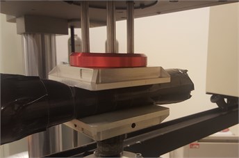
Fig. 12Relationship between contact force, displacement and pressure

The additional latex tube is connected to the PSE as shown in Fig. 4. The PSE is totally covered with tape so it can be assumed that change of the PSE volume caused by internal pressure is negligible and the total change of volume is completely caused by the change of volume of the additional latex tube.

Fig. 13Scheme of the latex tube with foam inserted inside

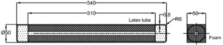
Fig. 14The scheme of the additional latex tube

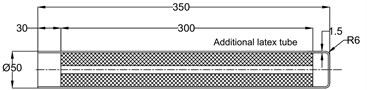
Firstly, we can use a simple calculation of volume of the PSE. The volume of the PSE is calculated in the way that is similar to the way and is given by:

28

V_{P S E} = π R^{2} l - V_{f o a m},

where: $R =$ 0.025 m is the radius of the PSE, $l =$ 0.3 m is the length of the PSE, $V_{f o a m} =$ 0.15 $l$ is the volume of foam (see Fig. 13).

Secondly, we consider the calculation of the volume of the additional latex tube. The additional latex tube is designed with the dimensions shown in Fig. 14. We can recognize that its structure is similar to the structure of the original PSE. The change of volume of additional latex tube depends on pressure $p_{s}$ and can be found experimentally. The setup of the experiment is shown in Fig. 15. At first the additional latex tube is filled with compressed air when the value of internal pressure meets the value of desired pressure. At second the additional latex tube is kept in a stable position and its surface is scanned by a 3D scanner machine.

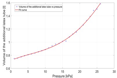
The calculation is programmed in Matlab software. The result is a set of volume values of the additional latex tube in the dependence of pressure. So the volume ( $V_{a d d}$ ) depending on internal pressure ( $p_{s}$ ) can be given in form of a polynomial function Eq. (29):

29

V_{a d d} = V_{a d d} (p_{s}) = k_{0} + k_{1} (p_{s} - p_{a t m}) + k_{2} {(p_{s} - p_{a t m})}^{2}

+ k_{3} {(p_{s} - p_{a t m})}^{3} + k_{4} {(p_{s} - p_{a t m})}^{4} - V_{f o a m} .

By using Matlab a set of coefficients is obtained as shown below:

k_{0} = 8.512599267236148 e - 04, k_{1} = 6.586794838689470 e - 09,

k_{2} = 4.111139460129753 e - 12, k_{3} = - 4.030675121010709 e - 16,

k_{4} = 1.163546770201630 e - 20 .

Fig. 15The setup of the experiment of the scanning of the surface of the additional latex tube

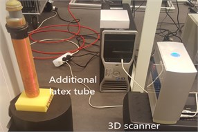
Fig. 16Example of a point cloud of the surface of the additional latex tube

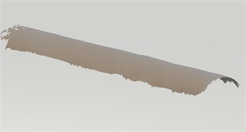
Fig. 17Volume-pressure diagram and the fit function

Finally, the total volume of latex air spring in the case of the improved system can be given by:

30

V_{i l s} = V_{i l s} (p_{s}) = V_{P S E} + V_{a d d} (p_{s}) .

Then the derivative of the total volume is:

31

{\dot{V}}_{i l s} = {\dot{V}}_{i l s} (p_{s}, {\dot{p}}_{s}) = \frac{d V_{a d d}}{d p_{s}} {\dot{p}}_{s} .

In summary, the mathematical model describing the improved system is given by first-order differential equations. For the purpose of using Matlab software, it is useful to transform this system of equations into matrix form:

32

\dot{X} = F (X),

where:

33

X = [\begin{array}{l} X_{1} \\ X_{2} \\ X_{3} \\ X_{4} \\ X_{5} \\ X_{6} \end{array}] = [\begin{matrix} x \\ \dot{x} \\ x_{d 1} \\ x_{d 2} \\ x_{d 3} \\ p_{s} \end{matrix}],

34

F (X) = [\begin{array}{l} F_{1} (X) \\ F_{2} (X) \\ F_{3} (X) \\ F_{4} (X) \\ F_{5} (X) \\ F_{6} (X) \end{array}] = [\begin{matrix} X_{2} \\ g - \frac{F_{f o a m} (X_{1})}{m} - \frac{F_{p} (X_{1}, X_{6})}{m} \\ {(\frac{1}{c_{1}} F_{d c} (X_{1}, X_{3}))}^{\frac{1}{n_{1}}} s g n (F_{d c} (X_{1}, X_{3})) + \dot{z} \\ {(\frac{1}{c_{2}} F_{d c} (X_{1}, X_{4}))}^{\frac{1}{n_{2}}} s g n (F_{d c} (X_{1}, X_{4})) + \dot{z} \\ {(\frac{1}{c_{3}} F_{d c} (X_{1}, X_{5}))}^{\frac{1}{n_{3}}} s g n (F_{d c} (X_{1}, X_{5})) + \dot{z} \\ \frac{κ q_{s} R_{g a s} T - κ X_{6} \frac{d V_{1} (X_{1})}{d X_{1}} (X_{1}) . X_{2}}{V_{l s} (X_{1}, X_{6}) + κ X_{6} \frac{d V_{3} (X_{6})}{d X_{6}}} \end{matrix}] .

The predefined functions of excitation $z$ , $\dot{z}$ , $\ddot{z}$ are continuous in an interval of time. The variable $q_{s}$ is calculated when the system of equations from Eq. (1) to Eq. (15) describing the function of the electro-pneumatic control subsystem is being solved. The solution of this system of equations gives as the results describing system response and system characteristics as kinematics of mass ( $x, \dot{x}, \ddot{x}$ ), pressure inside the PSE ( $p_{s}$ ) in case of mechanical subsystem, the flow rate $(q_{s}, q_{r}, q_{c,} q_{s 1}, q_{s 2}, q_{s 3}, q_{s 4})$ , pressure $(p_{c r}, e, \dots)$ , supplied coil current of proportional valves $i_{j}$ ( $j =$ 1, 2) in case of electro-pneumatic control subsystem and forces $(F_{f o a m}, F_{p}, \dots)$ , volume change of PSE ( $Δ V_{b}$ ), etc.

To solve the system of equations the initial and boundary conditions were provided. Initial conditions for the system of equations of the improved system are the values of the variables $x$ , $x_{d i}$ , $\dot{x}$ , $p_{s}$ , $q_{s i}$ , $q_{c}$ , $p_{c}$ , $V_{i l s}$ at time $t =$ 0 and boundary conditions for the system equations are the values of the parameters $p_{c r 1}$ , $p_{c r 2}$ , $p_{v r 1}$ , $p_{v r 2}$ , $e_{s}$ , $Δ p_{s}$ .

3. Calculation of the response of the improved system

The examples below show the behavior of the original system when it works under static conditions (without excitation $z (t)$ ) and dynamic conditions (with excitation $z (t)$ ) for both modes of operation (constant stiffness and constant pressure) and the load $m =$ 10 kg.

Fig. 18The calculated response of the improved system

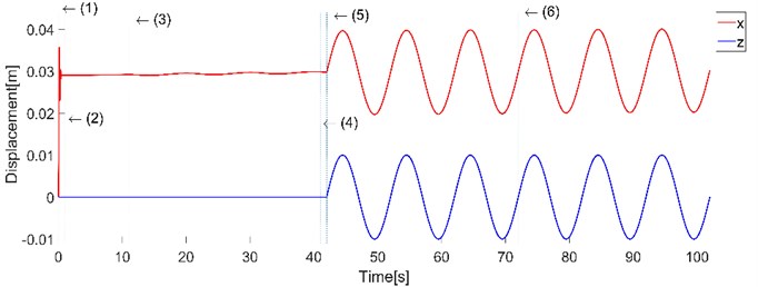
a) Displacement of mass $x$ and diplacement excitation $z$

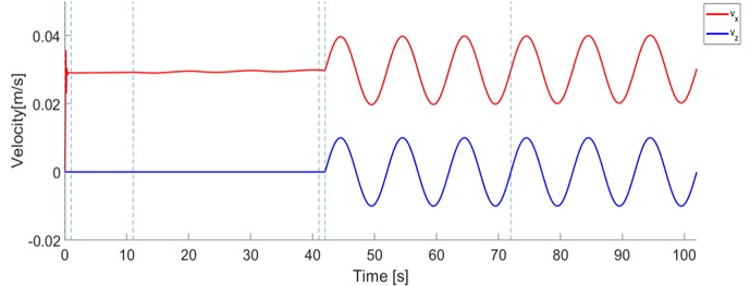
b) Velocity of mass $v x$ and velocity of excitation $v z$

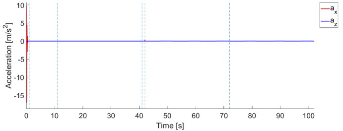
c) Acceleration of mass $a x$ and acceleration of excitation $a z$

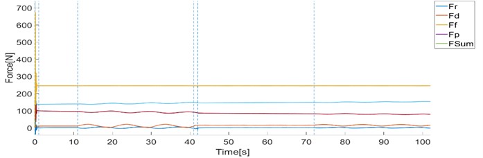
d) Forces

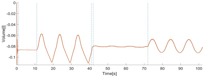
e) Volume change of latex air spring

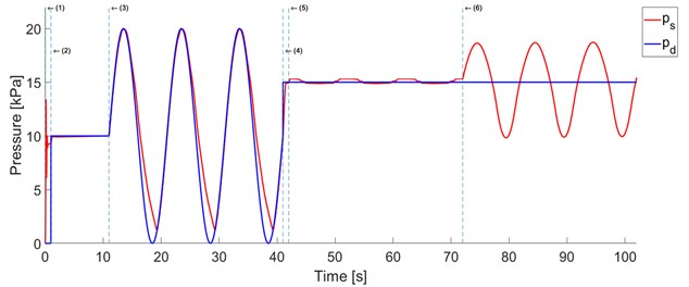
f) Pressure responce $p s$ and desired pressure $p d$

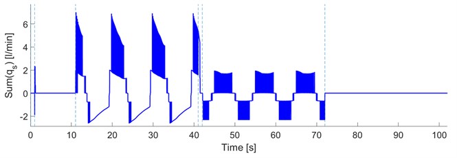
g) The flow rate qs through the PSE

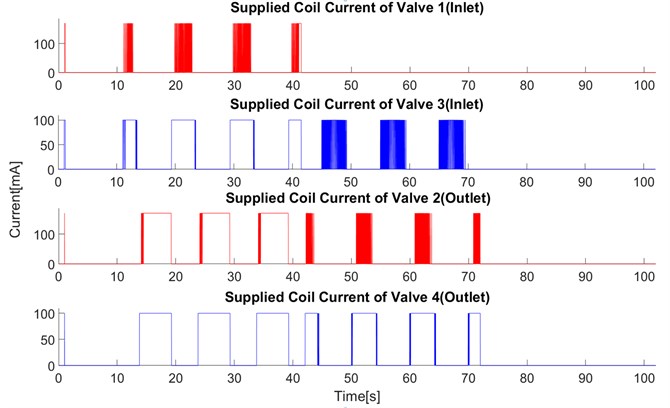
h) Supplied coil current of the valves $V_{1}$ , $V_{2}$ , $V_{3}$ , $V_{4}$

4. Calculation of transmission of acceleration

The transmission of acceleration is an important property of efficiency of vibration isolation systems. This is a way how to evaluate the influence of the PSE under dynamic conditions. In this article, we use the signal with continual change of frequency what is advantageous for investigation of nonlinear systems. For such cases so-called sweep sine functions are usually used. According to [8] the harmonic excitation function can be replaced by a sweep sine with variable frequency. Numerous human vibration studies conducted over the past several decades have shown that the human body is sensitive to low-frequency vibration occurring below 10 Hz [9]. Based on this the range was set to 1-11 Hz. The amplitude of acceleration was set to constant value of 0.1 g. The excitation function used for experiments under dynamic conditions is expressed in the form:

35

z (t) = Z_{a} {(t + t_{0})}^{2 (1 - n)} s i n (c {(t + t_{0})}^{n})

where: $n$ is the exponent of excitation function ( $n =$ 2), $f_{s t a r t}$ is start frequency, $f_{s t o p}$ is the stop frequency, $T$ is the total time of the excitation signal, $g$ is the gravitational acceleration and the other parameters are calculated as follows:

36

c = π \frac{f_{s t o p} - f_{s t a r t}}{T} 1 / s^{2},

37

t_{0} = {(\frac{2 π f_{0}}{n c})}^{\frac{1}{n - 1}} s,

38

Z_{a} = \frac{0.1 g}{n^{2} c^{2}} m / s^{2} .

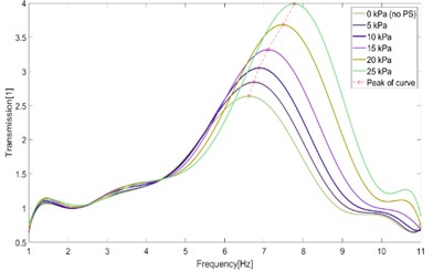
Fig. 19 and Fig. 20 show calculated results of the transmission of acceleration in case of using constant pressure mode and constant stiffness mode of control operation. The transmission curves are shown in cases of desired pressure $p_{d} \in$ {0, 5, 10, 15, 20, 25} kPa in dependence on the frequency of excitation in the range [1, 11] Hz. With a load of 10 kg, peaks of the transmission curves are positioned in the range of [6, 8] Hz and peak values are in range [2.5, 4].

Fig. 19Transmission of acceleration – constant pressure mode

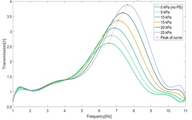
Fig. 20Transmission of acceleration – constant stiffness mode

5. Conclusions

The model of the original system consists of the model of foam block which is based on the article [6] and the model of a latex air spring and the model of electro-pneumatic control which are found experimentally. This model allows to investigate the response of the system to kinematic excitation or the change of the desired pressure inside pneumatic spring. Calculated results describe the behavior of characteristics of the improved system in detail when the improved system works in control modes (constant pressure and constant stiffness) and under static and dynamic conditions. The model is also used for evaluation of vibration isolation effect of the system which is possible to represent in form of the curves of transmission of acceleration. The transmission of acceleration shows the same tendency to shift the peak position toward the higher frequency when the desired pressure increases. This frequency shift is followed by simultaneous increase of peak value.

References

Cirkl D. Seat. Patent No. 303163, 2012.

Search CrossRef
Cirkl D., Tran Xuan T. Modelling of dynamical behavior of pneumatic spring-mass system. Engineering Mechanics Proceedings, Vol. 24, 2018, p. 865-868.

Search CrossRef
Cirkl D., Tran Xuan T. Simulation model of seat with implemented pneumatic spring. Vibroengineering Procedia, Vol. 7, 2016, p. 154-159.

Search CrossRef
Compact Proportional Solenoid Valve. Series PVQ, SMC catalog.

Search CrossRef
Port Solenoid Valve. Series S070, SMC catalog.

Search CrossRef
Cirkl D., Hrus T. Simulation model of polyurethane foam for uniaxial dynamical compression. Vibroengineering Procedia, Vol. 1, 2013, p. 53-58.

Search CrossRef
Cirkl D. Mechanical Properties of Polyurethane Foam. Ph.D. Thesis, Technical University of Liberec, Liberec, 2005.

Search CrossRef
Sivčák M. Dynamics of the Vibration Isolation System with More Degrees of Freedom. Ph.D. Thesis, Technical University of Liberec, Liberec, 2009.

Search CrossRef
Griffin M. J. Handbook of Human Vibration. Academic Press, London, 1990.

Search CrossRef

About this article

Received

05 December 2019

Accepted

19 December 2019

Published

30 June 2020

DOI

https://doi.org/10.21595/mme.2019.21211

Keywords

pneumatic spring

mathematical model

improved system

transmission of acceleration

This is an open access article distributed under the Creative Commons Attribution License, which permits unrestricted use, distribution, and reproduction in any medium, provided the original work is properly cited.

Next article in issue Next

Research article

2019 09 30

The effect of system improvement on regulation of pressure inside pneumatic spring element and on transmission of acceleration

Tien Tran Xuan, David Cirkl

Research article

2019 08 15

Multi-objective optimization of active suspension predictive control based on improved PSO algorithm

Qiang Zhao, Baoquan Zhu

Research article

2017 09 26

FEM model of pneumatic spring assembly

Tien Tran Xuan, David Cirkl

Research article

2016 11 15

Modeling and analysis of the vibration characteristics of a new type of in-arm hydropneumatic suspension of a tracked vehicle

Congbin Yang, Xiaodong Gao, Zhifeng Liu, Ligang Cai, Qiang Cheng, Caixia Zhang

T. Tran Xuan and D. N. Phu, “The mathematical model of the improved system of the seat with adjustable pressure profile,” Mathematical Models in Engineering, Vol. 6, No. 2, pp. 79–92, Jun. 2020, https://doi.org/10.21595/mme.2019.21211

Copy Extrica

Copied to clipboard!

TY  - JOUR
DO  - 10.21595/mme.2019.21211
UR  - https://doi.org/10.21595/mme.2019.21211
TI  - The mathematical model of the improved system of the seat with adjustable pressure profile
T2  - Mathematical Models in Engineering
AU  - Tran Xuan, Tien
AU  - Phu, Dong Nguyen
PY  - 2020
DA  - 2020/06/30
PB  - JVE International Ltd.
SP  - 79-92
IS  - 2
VL  - 6
SN  - 2351-5279
SN  - 2424-4627
ER  - 

Copy Ris

Copied to clipboard!

@article{Tran_Xuan_2020,
	doi = {10.21595/mme.2019.21211},
	url = {https://doi.org/10.21595/mme.2019.21211},
	year = 2020,
	month = {jun},
	publisher = {{JVE} International Ltd.},
	volume = {6},
	number = {2},
	pages = {79--92},
	author = {Tien Tran Xuan and Dong Nguyen Phu},
	title = {The mathematical model of the improved system of the seat with adjustable pressure profile},
	journal = {Mathematical Models in Engineering}
}

Copy Bibtex

Copied to clipboard!

[1]T. Tran Xuan and D. N. Phu, “The mathematical model of the improved system of the seat with adjustable pressure profile,” Mathematical Models in Engineering, vol. 6, no. 2, pp. 79–92, Jun. 2020, doi: 10.21595/mme.2019.21211.

Copy IEEE

Copied to clipboard!

Tran Xuan, Tien, and Dong Nguyen Phu. “The Mathematical Model of the Improved System of the Seat with Adjustable Pressure Profile.” Mathematical Models in Engineering 6, no. 2 (June 30, 2020): 79–92. https://doi.org/10.21595/mme.2019.21211.

Copy Chicago

Copied to clipboard!

The mathematical model of the improved system of the seat with adjustable pressure profile

Abstract

1. Introduction

2. Mathematical model

2.1. Model of the electro-pneumatic control subsystem

2.1.1. Model of the valves

2.1.2. Mathematical model of the compressed air supply

2.1.3. Mathematical model of the vacuum pump

2.2. Model of the mechanical subsystem

2.2.1. Model of polyurethane foam

2.2.2. Model of the combination of the latex air spring and the additional latex tube

3. Calculation of the response of the improved system

4. Calculation of transmission of acceleration

5. Conclusions

References

About this article

Related Articles