Abstract
We investigated the nonlinear elastic characteristic of an in-arm hydropneumatic suspension unit (ISU) as well as the damping characteristic of the controllable vane absorber. Due to the strong nonlinear characteristic of the ISU, simplify is needed to accurately model the vehicle. Based on the theory of multibody dynamics, a virtual prototype of the tracked vehicle was built, which includes the hydraulic system, the multi-dynamics of running gears and a road surface model. The virtual prototype is validated using both a static balancing test and a stiffness characteristics test. By simulating the road impact loading of the tracked vehicle when travelling on a trapezoidal US military road, the changes of the pitch angle and the acceleration of seats and centroid of the tracked vehicle was analyzed for two different damping ratios. We also determined key ride indicators for different speeds. The stiffness and damping characteristics of the ISU were tested in a bench experiment.
1. Introduction
The ISU is installed between the side walls of a tracked vehicle and the road wheel. This saves a good deal of interior space, while providing good nonlinear elastic properties and superior damping performance. Modeling and analysis of ISU are essential and the basis for smooth design and good suspension control.
In the 1970s, the ISU was used in tracked vehicles by the US Company National Waterlift, for the first time. It demonstrated superior damping performance, a compact structure and a substantial increase in mobility. In 2006, InARM® ISU, developed by Horstman Defence Systems in the UK, was successfully used for NLOS mobile artillery. In 2012, Horstman Defence Systems was selected to develop and ISU for the future chariot project by General Dynamics Land Systems [1-4]. The Korea Institute for Defense in cooperation with Tongmyung Heavy Industries Co. Ltd (Doosan Group) developed a type of ISU that was frequently used in XK-2 MBT and K21 APC, because of its excellent performance [5-8]. In 2010, India’s chariot R&D department of Ministry, CVRDE, developed a variation of the ISU for future APC. Multibody dynamic analysis of a tracked vehicle performed using LMS simulation software, includes superelement tracked vehicle analysis, detailed track analysis, and flexible body track analysis [9].
ISUs are widely used in heavy vehicles in the military. Researchers spent many years developing and improving a theory for ISUs. D.A. Crolla [10] analyzed and designed an active control system for a limited bandwidth ISU. Self-balancing of the actuator as well as a delay was included in the model, and a bench verification was conducted. Demerdash [11] designed a limited bandwidth ISU, which was based on a linear optimal control theory analyzed by a semi vehicle model simulation. It showed a significant improvement. F. Gay and Xavier Moreau [12-14] proposed a low-frequency control strategy for active hydropneumatic suspensions using both feedforward and feedback control.
In this paper, we investigated a Novel ISU. The output force of the hydropneumatic springs and suspension were computed and analyzed and the internal flow characteristics of the controllable vane absorber were investigated. Three different types of internal gap flow states of absorbers are discussed. The analytic relationship between opening and flow characteristics of adjustable damping valves was derived. We developed a damping model for a controllable vane absorber and a thermodynamic model of the ISU. Tracked vehicles are complex systems that contain many subsystems. Kinematic analysis based on classical mechanics and methods is generally difficult to perform [15]. Based on the theory of multi-body dynamics, we developed a tracked vehicle multi-body dynamics model, which reflects many aspects of the problem. The model includes the ISU model, track model, and a road contact model. The geometric and mechanical parameters were either identical or similar as the prototype vehicle. We conducted multi-body dynamic simulations of tracked vehicles with ISUs and evaluated the comfort level for the driver. The performance of the ISU was verified in a bench test.
2. Theory and empirical models
2.1. Elastic model
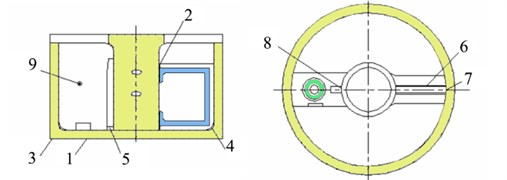
The ISU is mainly composed of an in-arm hydropneumatic spring (elastic member) and a controllable vane absorber (damping element) – see Fig. 1.
The in-arm hydropneumatic spring is composed of an actuating cylinder, a main piston, a piston connecting rod, a floating piston, a main plenum chamber, and a sub plenum chamber. The actuating cylinder is integrated with a balance elbow. One end of the piston connecting rod is hinged on a support arm in the suspension, while the other end is connected to the main piston via a ball joint.
Fig. 1Schematic of ISU
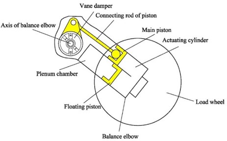
Fig. 2Structure and dimensions of the ISU
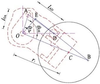
To facilitate the kinematic analysis of the mechanism inside an ISU, we simplified it into a planar system – see Fig. 2. Point O is the balance elbow axis of the ISU. Point A is the top of the piston connecting rod. Point B is the intersection of the actuating cylinder centerline and the balance elbow. Point C is the axle of the road wheel. Point D is the center of the sphere of the rod connecting the pistons. OE is the radius of action of the actuating cylinder. Geometric parameters of the ISU are shown in Table 1.
If wheel travel is and the static angle is known as , the angle of balance elbow is:
is the distance of point E from the radius of gyration, and the coordinates of each point can now be calculated as follows.
Table 1Geometric parameters of the ISU
No. | Items | Unit | Symbol |
1 | Length of upper arm | mm | |
2 | Angle of upper arm and horizontal | ° | |
3 | Length of connecting rod | mm | |
4 | Arm of actuator cylinder | mm | |
5 | Mounting angle of radius of action of actuator cylinder | ° | |
6 | Radius of gyration of the balance elbow | mm | |
7 | Static stroke | mm | |
8 | Dynamic stroke | mm | |
9 | Distance of balance elbow rotation center from bottom | mm | |
10 | Body height of track shoe | mm | |
11 | Vehicle body height from the ground | mm | |
12 | Road-wheel diameter | mm | |
13 | Rubber deformation amount of road-wheel and track-shoe surface | mm |
Coordinates of Point E:
Coordinates of Point C:
Coordinates of Point B:
Coordinates of Point D:
where:
The derivatives of Point B with wheel travel are:
The derivatives of Point E with wheel travel are:
The derivatives of Point D with wheel travel are:
The position of the actuator cylinder piston is , and the piston position when the main plenum chamber pressure reaches the sub plenum chamber pressure is . To obtain the coordinates of the movement of piston, we use:
When 0, the main plenum chamber and sub plenum chamber work at the same time. When 0, only the main plenum chamber works.
The output force of the hydropneumatic spring analysis is:
(1) When only the main plenum chamber works, 0, the gas changeable index 1, and the hydropneumatic spring pressure to meet is:
where, and are volume and pressure of the main plenum chamber when 0, respectively.
where, is the gas height of the main plenum chamber when 0. When:
then the output force of the hydropneumatic spring is:
where, is the diameter of the actuating cylinder.
Then hydropneumatic spring stiffness is:
(2) When, the main plenum chamber and sub plenum chamber work at the same time, 0:
Here, is the commuted column height of the main plenum chamber after considering the inflatable volume of the piston in the sub plenum chamber. is the diameter of the main plenum chamber. is the diameter of the sub plenum chamber.
Then pressure, output force and stiffness of the hydropneumatic spring are:
The output force of the suspension analysis is calculated as follows:
The vertical load of each wheel suspension is:
For Point O:
Therefore, the force on the main piston with the connecting rod is:
The output force of the actuating cylinder is:
The lateral pressure on the actuating cylinder from main piston can now be obtained:
The ISU workspace was selected to have 0-200 mm wheel travel range.
The connecting rod force derivation of wheel travel is:
For Point O:
the suspension force is:
The derivation of wheel travel is:
Therefore, we obtain the suspension stiffness:
The formula is the final expression of the suspension stiffness equation.
2.2. Damping model
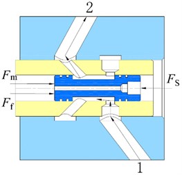
As shown in Fig. 3, the controllable vane absorber is in-arm, coaxially arranged with the balance elbow shaft, and connected via a spline. It mainly consists of a blade shaft, a pressure-limiting valve, a damper adjusting device, and partitions. The damping force from absorber fluid flowing through pores repeatedly consumed vibration energy [16].
The vane damper flow can be obtained using the following formula:
where, is tangential velocity of the absorber connecting arm outer end, is the connecting arm length, is the height of the vane, , are the inner and outer diameters of the vane.
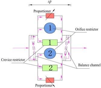
Fluid structure diagram of the controllable vane absorber is shown in Fig. 4. Since the flow values and structure parameters of two pressure-equalizing oil pipelines are equal, the pressure differences are equal too. The pressure difference between the No. 1 and No. 2 oil pipeline is set to . Flow through the No. 1 and No. 2 oil pipeline is set to and , Since the upper and lower oil pipeline structures are exactly the same, we can write:
Fig. 3Schematic of the controllable vane absorber
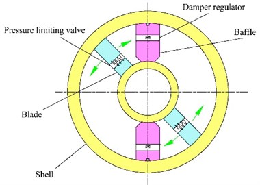
Fig. 4Fluid schematic of controllable vane absorber
Major gaps of the controllable vane absorber are shown in Table 2 and Fig. 5.
Table 2Major gaps of the controllable vane absorber
No. | Amount | Structure | Relative movement between contact surfaces | Remarks |
1 | 2 | Straight | No | Separator bottom and case |
2 | 2 | Curved | Yes | Blade seals and blade shaft |
3 | 2 | Curved | No | Separator bottom and case |
4 | 2 | Curved | Yes | Vane seals and case |
5 | 2 | Straight | No | Blade seals and case |
6 | 2 | Straight | Yes | Produced by vane seal flatness |
7 | 2 | Straight | Yes | Produced by vane seal straightness |
8 | 2 | Straight | No | Produced by Blade seal flatness |
9 | 2 | Hole | No | Constant throttle orifice |
10 | 2 | Hole | No | Constant throttle orifice |
Fig. 5Structure and gaps of the controllable vane absorber
The circular section pipe Reynolds number is calculated as:
where, is the liquid average velocity in the pipeline, is the pipe diameter, is kinematic viscosity value of the liquid.
To simplify the calculations, the equivalent hydraulic diameter is used instead of the pipe diameter. The non-circular cross-section is assumed circular. The equivalent hydraulic diameter is calculated as:
where, is the real overcurrent sectional area of the pipe, is the wetted perimeter of the pipeline.
There is a relationship between dynamic viscosity and kinematic viscosity of incompressible fluids: , the Reynolds number of the non-circular cross-section linear pipeline can be calculated using the following formula:
The state of oil flow can be determined according considering the critical pressure. From the calculation, the liquid flow state of the No. 1 gap is laminar flow, and the one of No. 5, No. 6, No. 7, No. 8 gaps are turbulent flow.
The pressure limiting valve constant throttle orifice, the No. 9 gap, belongs to a second category, because constant throttle orifices are designed as a ladder long hole with secondary throttling. When the pipe cross-section experiences sudden changes, there will be a sudden increase in the velocity of the liquid, causing a voltage drop at the same time. The flow state is very complex, as it constitutes turbulent flow.
The vane absorber is a rotary structure, which includes many parts. The contact gap of these parts – No. 2, No. 3, No. 4 is elbow-shaped. Most of these gap sections are irregular shapes. Due to centrifugal force, fluid interacts with the pipeline wall, which leads to a swirl. When this occurs in such gaps this creates a typical turbulent state.
The vane absorber can be adjusted by opening the electro-hydraulic proportional valve, which, in turn, adjusts the damping force. The structure diagram of an electro-hydraulic proportional valve is shown in Fig. 6.
Using Bernoulli’s equation, we can formulate the relationship between the valve inlet and outlet:
where, for same valve opening, the total loss of flow in the proportional control valve is a function of the flow through the valve .
Fig. 6Structure diagram of an electro-hydraulic proportional valve
Since the flow entrance areas are equal, , the relationship between flow and pressure difference of the proportional control valve can be determined:
For a given opening of the proportional control valve, the relationship between flow and pressure difference is:
For the same pressure difference, the proportional flow valve flow coefficient is only related to the valve opening (1-4 mm). There is no temperature derating. According to the relationship between pressure difference and flow rate of test, the parameter of Eq. (37) was fitted.
Table 3 shows when the valve pressure difference is 7 MPa, the parameter for different valve openings. This was fitted as shown in Table 3.
Table 3Fitted values of cv for different degrees of valve openings
Opening degree / ×10-3 (m) | 0 | 0.1 | 0.5 | 1 | 1.5 | 2 | 2.5 | 3 | 3.5 | 4 |
Parameter /×10-9 | 0 | 0.01 | 0.059 | 0.12 | 0.17 | 0.19 | 0.21 | 0.22 | 0.23 | 0.24 |
Flow / (l/min) | 0 | 3.2 | 23.7 | 50.4 | 71.4 | 79.8 | 88.2 | 92.4 | 96.6 | 100.8 |
According to our analysis, the flow in a planar gap in the controllable vane absorber is turbulent. The flow rate can be calculated as:
The constant flow in the throttle orifice is calculated as:
Flow and in chamber 1 and 2 are:
where, and are the comprehensive flow parameters in the turbulence model. considers flow due to the pressure difference in the controllable vane absorber, and is the ratio of shear flow in a controllable vane absorber. is the comprehensive turbulent flow coefficient, which is constant at same temperature.
According to the principle of balanced moments, the damping force at the outer end of the shock absorber connecting arm is:
where, is the pressure difference between the high and low pressure chamber.
Finally, the damping model of the controllable vane absorber can be formulated:
When the oil temperature increases, viscosity decreases, and the flow rate in the shock absorber increases at the same pressure. Therefore, the parameters , and increase with increasing temperature, which reflects the shock absorber damping force decline. As a result, turbulence is easier to form when the temperature increases.
The proportional control valve of the internal oil passage is complex. Assuming that the working oil is incompressible, one can consider the impact of the mass force, and the flow of working oil in the proportional valve needs to satisfy the following formula:
The Reynolds control equation for turbulent flow [17] is:
where, is the density of the fluid, is the Reynolds stress, , , are the mean velocity, the mean mass force and the mean pressure, , are values of the fluctuating velocity.
The turbulent energy equation [17] can be formulated as:
where, is the kinetic energy for turbulent pulsating, is the dissipation rate for the turbulent energy equation, is the kinematic viscosity of the working oil.
Incompressible turbulent flow is usually described as - model [17]:
where, is the generating term of turbulent energy, 0.09-0.11.
According to the relationship between shock absorber damping force and excitation speed determined by bench testing, the parameter identification for the damping characteristics analysis formula of the shock absorber turbulence model was conducted. The damping force of vane damper follows a normal distribution. The expected values of the experimental data for each damper were taken as the fit data. We used the least squares method to determine the parameters for the prototype vane damper – see Table 4.
Table 4Parameters for the prototype vane damper
Temperature | ||||
30 °C | –0.0263×10⁶ | 0.0035×10⁶ | 0.2616×10⁶ | –1.1180×10⁶ |
50 °C | –0.0665×10⁴ | 0.0094×10⁴ | 0.5889×10⁴ | –2.7477×10⁴ |
80 °C | –0.0462×10⁴ | 0.0066×10⁴ | 0.4134×10⁴ | –1.5006×10⁴ |
110 °C | –0.0900×10⁴ | 0.0138×10⁴ | 0.1312×10⁴ | –2.1235×10⁴ |
140 °C | –0.4644×10³ | 0.0591×10³ | 3.7299×10³ | –3.8257×10³ |
When the temperature increases, oil viscosity decreases. For the same pressure, the flow through the damper gap increases, which indicates that as the temperature rises, and the downward trend of the shock absorber damping force increases. As a result, the formation of the internal flow field turbulence becomes easier.
3. Multi-body dynamic analysis
3.1. Modeling
The ISU of a tracked vehicle is a complex multi-body nonlinear system. Traditionally researchers use a simplified model. Simplified models are often based on assumptions, and the accuracy of the model can therefore become low. In this paper, LMS Virtual Lab Motion was used in multi-body dynamics analysis to address this problem.
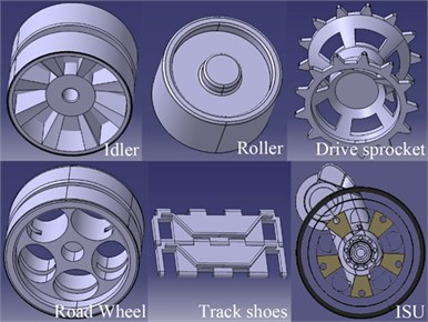
The structural parameters of a tracked vehicle as the basis, discrete track toolkit of LMS Virtual Lab was used to develop a tracked vehicle driving system simulation model – see Fig. 7.
Fig. 7CAD models of the components of the driving system
When the Young modulus of a contact surface is not 0, the calculation of contact forces can be performed using the Hertz contact formula [18]:
where:
and is the penetration depth. is the maximum penetration depth. , are the maximum and minimum radiuses of curvature at the first point of contact. , are the maximum and minimum radiuses of curvature at the second point of contact. , are Young’s moduli of two objects. , are the Poisson’s ratios of two objects. is the conversion speed. is the angle between two surfaces.
Various types of contacts can be reduced to Point-to-Point contact, Sphere-to-Extruded-Surface contact, Sphere-to-Revolved-Surface contact, Extruded-Surface-to-Revolved-Surface contact, and Sphere-to-Ground contact.
The contact of the drive sprocket teeth and the track shoe was set to Sphere-to-Extruded-Surface contact. To prevent detachment, lateral constraints were added. The contact of idler and track were divided into two types: One is the contact of idler and track shoe board, the other is the wheel side and track shoe teeth. Contact between track and ground was defined via Sphere-to-Ground contact.
The digital terrain model was output using meshes – see Fig. 8.
Fig. 8Digital terrain model
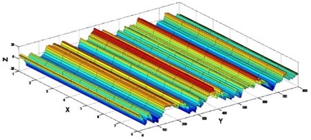
A precise model for soft ground was used in this simulation, and a “memory” feature for soil was considered. This modeling approach took into account the coupling of tracks on the ground. The mechanical property parameters of soil were used as listed in Table 5.
Table 5Mechanical parameters of soil
Parameters | Units | Values |
Elastic Modulus | MPa | 20.5 |
Critical deflection | m | 9.9×10⁻³ |
Cohesive modulus | kN/mn+1 | 41.7 |
Friction modulus | kN/mn+2 | 1466 |
Exponent of the sink equation | 0.57 | |
Poisson’s ratio | 0.24 | |
Cohesion of the regolith | kPa | 6.07 |
Angle of internal friction | rad | 0.46 |
The ISU hydraulic model was developed at LMS Imagine Lab AMESim, which was divided into four parts: actuating cylinder, accumulator, main valve, and pressure relief valve. The floating piston mass was taken into account in the AMESim equivalent model of the ISU accumulator. The stiffness and damping of the stopper, when ISU was punctured, was defined as shown in Fig. 9.
Fig. 9The ISU hydraulic model
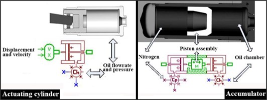
Fig. 10Tracked vehicles simulation model
Finally, the multi-body dynamic model of a tracked vehicle was jointly developed by LMS Virtual Lab Motion and LMS Imagine Lab AMESim, which includes the following components: hull, road wheel, sprocket, idler, roller, ISU, Track system and Tensioner – see Fig. 10.
The constraint relationships between the components are shown in Table 6.
Table 6Constraint relationships between components
Component 1 | Component 2 | Joint types |
Road wheel | ISU | Rotation joint |
ISU | Hull | Rotation joint |
Roller | Hull | Rotation joint |
Sprocket | Hull | Rotation joint |
Idler | Hull | Rotation joint |
Tensioning device 2 | Hull | Cylindrical joint |
Tensioning device 1 | Connecting rod | Cylindrical joint |
Prior to the vehicle dynamics simulation, two methods were used to verify the model’s accuracy. Static equilibrium angles of road arms were compared with the actual vehicle, and the differences do not exceed 3.4 %. Also the simulation and the mathematical model predictions of road wheel travel and the hydropneumatic spring were compared. The differences do not exceed 2.8 %.
We analyzed the impulse response of a tracked vehicle for different suspension damping ratios and a road with continuous obstacles.
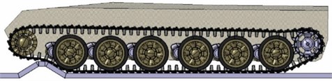
The simulation road was a 60 m long road with six US military standard trapezoidal obstructions (10 inches tall) at irregular intervals – see Fig. 11.
The simulation speed was the maximum off-road speed of the tracked vehicle (40 km/h).
Evaluation: The vertical acceleration at the driver’s seat is near or below 2.5 g, which defines the condition for the driver to endure.
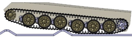
Details of the simulations of high-speed obstacle clearance of the tracked vehicle are shown in Fig. 12.
Fig. 11The road with the standard obstacles
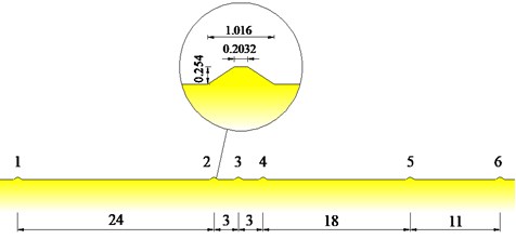
Fig. 12Simulation of high-speed obstacle-clearance of the tracked vehicle
3.2. Simulation results
Figs. 13-15 show time domain curves for vertical vibration acceleration at the driver’s seat , vehicle centroid vertical acceleration , and vehicle pitch angle acceleration for different suspension system damping ratios with trapezoidal obstacles at 40 km/h speed.
Fig. 13Time domain curve of the vertical acceleration of the driver’s seat
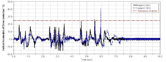
Fig. 14Time domain curve of the vehicle centroid vertical acceleration
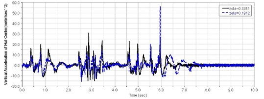
Fig. 15Time domain curve of the vehicle pitch angular acceleration
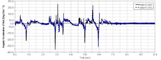
Fig. 16The first balance elbow corner
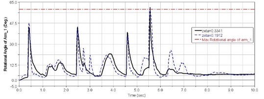
Fig. 17The second balance elbow corner
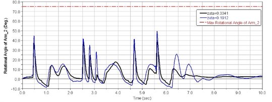
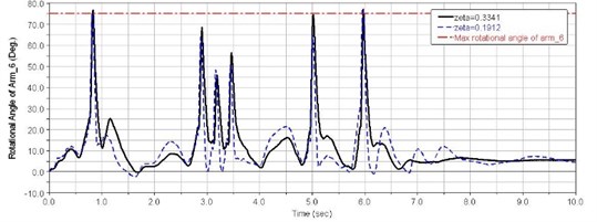
Figs. 16-18 show impulse responses of first, second and sixth balance elbow corners for different suspension systems damping ratio with trapezoidal obstacles at 40 km/h speed.
Fig. 18The third balance elbow corner
3.3. Analysis of the simulation results
(1) When 0.35 s, as shown in Fig. 15, the first road wheel hits the first trapezoid obstacle, causing a sharp increase in the first balance elbow corner, and the driver's seat vertical acceleration is reflected in the first peak 18.6 m/s2. At this moment, the first balance elbow did not hit the stopper.
(2) When 0.8 s, as shown in Fig. 19, the sixth road wheel hit the first trapezoid obstacle. At this moment, the sixth balance elbow struck the stopper, and the vehicle was affected by puncturing of the suspension. The driver’s seat vertical acceleration appeared as a second peak 10.6 m/s2.
(3) When 1.12 s, the first, second, and sixth road wheel received a second shock from ground after over the obstacle, and driver’s seat vertical acceleration appeared the third peak 15.6 m/s2.
(4) When 2.45 s-3 s, as shown in Fig. 15, the first road wheel hit the second trapezoid obstacle, the first balance elbow did Not strike the stopper. In the following 0.5 seconds, the first road wheel hit the third and fourth trapezoid obstacle continuously. The driver's seat vertical acceleration appeared 3 peaks. 16-17 m/s2. Large changes of vehicle pitch angular acceleration appeared during this time, as shown in Fig. 16.
(5) When 4.6 s, the first road wheel hit the fifth trapezoid obstacle. Due to large vehicle pitch angular acceleration, the shock response was significant, and 22.9 m/s2.
(6) When 5.56 s, the first road wheel hit the sixth trapezoid obstacle. Due to dual role of a second shock over fifth trapezoidal obstacle and pitch vibrations, the first balance elbow struck the stopper, and the shock response of the driver’s seat reaches a very large value. When 0.19, 26.2 m/s2. At this point, the vertical vibration acceleration at the driver’s seat exceeded the human tolerance limit. In other words, the suspension damping ratio needs to improve.
(7) When 5.95 s, the sixth road wheel hit the sixth trapezoid obstacle. Due to the sixth balance elbow striking the stopper, the shock response of the driver’s seat reaches its highest value when 0.19 and 40.6 m/s2. In this case, the vehicle centroid vertical acceleration was very large too, as shown in Fig. 15. The reason for this is that the vibration frequency is close to the natural frequency of the vehicle. When the suspension damping ratio 0.33 and 15.5 m/s2, the vertical vibration acceleration at the driver’s seat wound still be below the human tolerance limit.
3.4. Effect of the suspension damping ratio on the shock response
(1) When the balance elbow does not hit the stopper.
When the tracked vehicle travels between the first and fifth trapezoidal obstacle, as shown in Table 7, smaller suspension damping causes lower vertical accelerations of the driver’s seat.
Table 7Driver’s seat vertical acceleration for maximum and minimum damping ratios (m/s2)
0.35 s | 0.8 s | 1.12 s | 2.45 s | 4.6 s | |
0.33 | 18.6 | 10.6 | 15.6 | 16.7 | 22.9 |
0.19 | 11.5 | 6.4 | 7.0 | 10.6 | 10.8 |
As shown in Figs. 16-18, when suspension damping is low, the range of the balance elbow rotational angle is greater, and can take full advantage of the suspension dynamic travel. This results in better comfort for the driver.
(2) When the balance elbow strikes the stopper.
Smaller suspension damping causes an increased probability of suspension puncturing. When suspension breakdown occurred, the vehicle riding comfort was greatly reduced. The driver’s seat vertical accelerations for different damping ratios in the moment the balance elbow strikes the stopper are shown in Table 8.
Table 8Driver’s seat vertical acceleration for maximum and minimum damping ratios (m/s2)
5.56 s | 5.59 s | |
0.33 | 24 | 15.5 |
0.19 | 26.2 | 40.6 |
Simulation results show that, when 0.33, the driver’s seat vertical acceleration stays within the human tolerance limit.
An ISU reference model with limited bandwidth active suspension and an active control algorithm was designed. The output for dynamic travel using the skyhook reference model is the track target, and a fuzzy PID control algorithm is used to track the moving stroke. The reference skyhook model for a virtual prototype model is shown in Fig. 19.
Fig. 19The reference skyhook model of a virtual prototype model
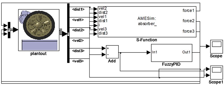
Measured road data was imported into the model. The road wheels were excited by vibration. The obtained dynamic travelling data were dealed using a 2 Hz low-pass filter as tracking target data for the control model.
4. Experiments
4.1. Experiment profile
The ISU performances were verified using a single wheel suspension test bench, which includes elastic force, damping force as well as the adjustment range of the damping force – see Fig. 20.
The ISU test platform was setup on a road simulator bench. The road simulator would simulate a variety of pavements. The bench was equipped with tension sensors to measure the force between the ISU and the bench but also with temperature sensors used to monitor the internal fluid temperature of the shock absorber.
Test schemes:
(1) The damping characteristic test conditions were the following:
Control currents, 0 A, 0.5 A, 0.8 A, 1.0 A, 1.2 A, and 1.5 A; amplitude, ±80 mm; frequencies, 0.955 Hz; sinusoidal excitation; fluid temperature shock absorber temperatures, 30 ℃, 50 ℃, 80 ℃, and 140 ℃.
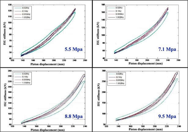
(2) The stiffness characteristic test conditions were the following: sub plenum chamber inflation pressure, 11 Mpa; main plenum chamber, 5.5 MPa, 7.1 MPa, 8.8 MPa, and 9.5 MPa; frequencies, 0.02 Hz, 0.1 Hz, 0.955 Hz, and 1.952 Hz; sinusoidal excitation.
Fig. 20ISU bench schematic

4.2. Test results and analysis
(1) Damping characteristics test.
Fig. 21 shows the ISU dynamometer cards at different temperatures and different control currents. We can see that, as the temperature increased, the shock absorber damping power is reduced, and shock absorber damping effect is reduced too. At the same time, the change range of the shock absorber damping force is significantly reduced, which indicates that the adjustment range of the damping force decreased.
Fig. 21ISU dynamometer card at different temperatures
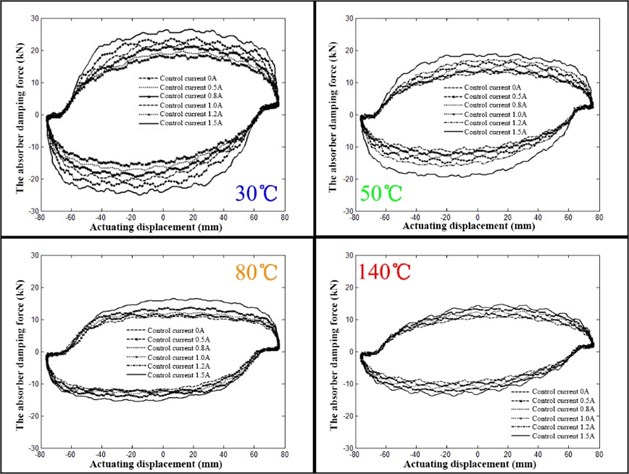
Table 9ISU damping force at different control currents and temperatures (kN)
Temperatures \ Control currents | 0 A | 0.5 A | 0.8 A | 1.0 A | 1.2 A | Adjustment range of damping force |
30 °C | 17.5 | 19.2 | 20.1 | 22.2 | 24.3 | 38.9 % |
50 °C | 15.9 | 16.3 | 17.9 | 18.8 | 20.5 | 28.9 % |
80 °C | 12.3 | 12.9 | 13.7 | 15.2 | 16.5 | 34.1 % |
140 °C | 10.2 | 10.9 | 11.5 | 12.3 | 13.0 | 27.5 % |
Table 9 shows the ISU damping forces at different control currents and temperatures.
1) The adjustment range of the ISU damping force continually decreased with increasing temperature. When the temperature was 30 ℃, the adjustment range could reach 38.9%, and at 140 ℃, it still reached 27.5 %.
2) Temperature between 50 ℃ and 80 ℃, the temperature attenuation ratio of the absorber damping force are 19.1 % and 23.5 %, which meets the design requirement of the shock absorber: Temperature from 50 ℃ to 80 ℃, temperature attenuation ratio should be less than 30 %.
(2) Stiffness characteristics test.
The ISU stiffness characteristics are shown in Fig. 22.
The ISU output stiffness increased with both increasing sinusoidal excitation frequency and increasing initial inflation pressure. Because of the dynamic friction, the curves for compression and rehabilitation stroke do not coincide. When the frequency is greater than 0.1 Hz, the dynamic characteristic without damping at different frequencies was similar. With increasing test time, the cylinder wall temperature did not rise, and dynamic friction is reduced.
Fig. 22ISU stiffness characteristic curves at different pre-charge pressures
The ISU output stiffness increased with both increasing sinusoidal excitation frequency and increasing initial inflation pressure. Because of the dynamic friction, the curves for compression and rehabilitation stroke do not coincide. When the frequency is greater than 0.1 Hz, the dynamic characteristic without damping at different frequencies was similar. With increasing test time, the cylinder wall temperature did not rise, and dynamic friction is reduced.
5. Conclusions
By studying the structure and working principles of an ISU, we were able to derive analytical formulas for the movement of ISU parts. This was done during a tracked vehicle engineering project. Based on a two-chamber hydropneumatic spring model, the output powers of the ISU were calculated and analyzed. We also performed an internal flow characteristics analysis of another important component of an ISU, the controllable vane absorber. The fluid states of three types of internal gaps of shock absorbers were analyzed. We developed an analytic relationship between the adjustable damping valve opening, flow characteristics and the damping characteristics model of the controllable vane absorber. Based on the theory of multi-body dynamics, using the commercial software LMS Virtual Lab Motion and LMS Imagine Lab AMESim, a multi-body dynamics model of tracked vehicles was developed. In addition, we also developed a soft ground model based on Bekker theory. The impact, when a tracked vehicle travels on a trapezoidal road, was simulated and analyzed. Changes in acceleration and pitch angles of both the vehicle seat and centroid were analyzed. Using an ISU bench test, the stiffness and damping characteristics of the ISU were also examined.
References
-
Davis L. W. In-arm Compressible Fluid Suspension System. Patent, 2010.
-
Stockford B. Suspension Unit. Patent, 2010.
-
Holman T., D’Aubyn R. Suspension Unit. Patent, 2011.
-
Holman T., D’Aubyn R. Suspension System. Patent, 2011.
-
Song Ohseop, Park Byunghoon A Study on the Dynamic characteristics of hydropneumatic suspension unit considering the nonlinear effects. Korea Society for Noise and Vibration Engineering, Vol. 17, Issue 8, 2007, p. 747-756.
-
Kim Byung Chul Development of Composite Spherical Bearing. Korea Advanced Institute of Science and Technology, 2008.
-
Han Insik Durability improvement of high pressure seal for ISU under the track vibration. Transactions of KSAE, Vol. 17, Issue 2, 2009, p. 112-117.
-
Park Dong Chang, Lee Seung Min, Kim Byung Chul, et al. Development of heavy duty hybrid carbon-phenolic hemispherical bearings. Composite Structures, Vol. 73, Issue 1, 2006, p. 88-98.
-
Shankar R. Future combat systems for futuristic infantry combat vehicles. Technology Focus, Vol. 18, Issue 5, 2010, p. 1-7.
-
Crolla D. Analysis and design of limited bandwidth active hydropneumatic vehicle suspension systems. Proceedings of the Automotive Dynamics and Stability Conference, 2000, p. 189-198.
-
El-Demerdash S. M. Performance of limited bandwidth active suspension based on a half car model. SAE Technical Paper, 1998.
-
Gay F., Coudert N., Rifqi I., et al. Development of Hydraulic Active Suspension with Feedforward and Feedback Design. SAE Technical Paper, Detroit, MI, United States, 2000.
-
Moreau Xavier, Rizzo Audrey, Oustaloup Alain, et al. Improvement of hydractive suspension hard mode confort thanks to a low frequency active CRONE system. Part 1: Problematics, strategy and modelling. 7th International Conference on Multibody Systems, Nonlinear Dynamics, and Control, Vol. 4, 2009, p. 1077-1086.
-
Moreau Xavier, Rizzo Audrey, Oustaloup Alain, et al. Improvement of hydractive suspension hard mode confort thanks to a low frequency active crone system. Part 2: control part and simulation results. 7th International Conference on Multibody Systems, Nonlinear Dynamics, and Control, Vol. 4, 2009, p. 1087-1094.
-
Kotb Ata Wael Galal Mohamed Intelligent Control of Tracked Vehicle Suspension. 2014.
-
Nirala S. K., Subash M. U., et al. Development of Hydro Gas Suspension for AFV: A Co-Simulation Approach. 2012.
-
Zhang Mingyuan, Jing Sirui, Li Guojun. Advanced Engineering Fluid Mechanics. Xi’an Jiaotong University Press, 2006.
-
Young W. C., Budynas R. G. Roark’s Formula for Stress and Strain. Seventh edition, McGraw Hill, 2002.
Cited by
About this article

This work was supported by the National Natural Science Foundation of China (51575009), China’s Post-doctoral Science Fund (2015M580947), Jing-Hua Talents Project of Beijing University of Technology, and the Project supported by Beijing Postdoctoral Research Foundation (2016ZZ-15).
Congbin Yang is the first author of the paper and completed the major work of writing. Xiaodong Gao is responsible for virtual prototype of the tracked vehicle. Zhifeng Liu is the corresponding author and responsible for nonlinear elastic characteristic of the in-arm hydropneumatic suspension unit. Ligang Cai is responsible for damping characteristic of the controllable vane absorber. Qiang Cheng is responsible for the bench experiment. Caixia Zhang is responsible for analysis of test results.
