Automated set-up parameter estimation and result evaluation for SSI-Cov-OMA

1. Introduction

Stochastic subspace identification is a widely used method to extract modal parameters from vibration data. In this context, two methods can be distinguished, namely the data-driven (Data-SSI) and covariance-driven (Cov-SSI) method. This paper will present an automated algorithm based on the Cov-SSI method. In general, the automation of Cov-SSI concerns two main steps. First of all, the model order and the number of block rows must be set as input parameters. The most common way to analyze a system is to create stability plots and search for the eigenfrequencies as vertical alignments of poles over many different model orders. Since the optimal number of block rows cannot be received analytically, stability plots for wide range of block rows are created. For this step, a peak-picking approach is used to set proper values for input parameters. The second main step of automation regards the interpretation of the stability plots. Each stability plot is analyzed via a hierarchical clustering method and the results are used in a sensitivity analysis to find the optimal value of block rows. A description of this principle can be found in [2]. Besides the common order reduction method, the algorithm uses the alternative method proposed in [1]. While the common method reduces the order of the Hankel matrix after the SVD, the modified method interchanges the sequence. Therefore, this paper also provides a brief comparison between both methods.

2. Basic description of Cov-SSI

First, we would like to provide a brief overview over the method, a more comprehensive description can be found in [3]. The Cov-SSI method is based on the assumption that a mechanical system can be transformed into its state space formulation defined by the State Space Equation in Eq. (1) and the Measurement Equation in Eq. (2):

With this, one defines the following identities for the Output covariance matrix ${\mathbf{R}}_i$ and the State output covariance matrix $\mathbf{G}$:

By assuming that all other relevant variables are not correlated with each other, Eq. (3) can be formulated as in Eq. (5):

The Output covariance matrices ${\mathbf{R}}_i$ for different values of $i$ describing the respective block rows of the covariance are used to construct a block Hankel matrix of covariances Eq. (6):

The dimension of the $p\times p$ block Hankel matrix depends on the number of sensors and the number of block rows used and is determined by Eq. (7):

Decomposing the block Hankel matrix of Eq. (6) by using the singular value decomposition yields the matrices $\mathbf{U}$, $\mathbf{S}$ and $\mathbf{V}$, where $\mathbf{S}$ contains singular values in decreasing order Eq. (8):

In general, all singular values will be larger than 0 due to unavoidable noise influences. In order to construct a stability plot for multiple model orders an order reduction according to the respective model order $k$ is performed. The System matrix ${\mathbf{A}}_d$ is then obtained by Eq. (9):

The matrix ${\left({\mathbf{H}}_{\alpha ,\beta }\right)}_1$ is constructed by shifting ${\left({\mathbf{H}}_{\alpha ,\beta }\right)}_0$ by one block row. By calculating the eigenvalue decomposition of the discrete System matrix ${\mathbf{A}}_d$ modal parameters are obtained.

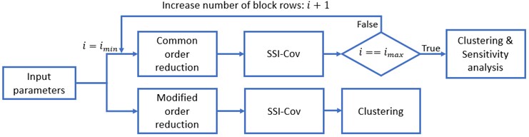
3. The algorithm

The first step of the algorithm is the determination of proper input parameters. Based on the two order reduction methods, the algorithm splits into two branches, Fig. 1. The upper one utilizes the common order reduction method. As stated before, this means the actual order reduction of the Hankel matrix takes place after the singular value decomposition. Therefore, the number of block rows influences the matrix given to the SVD. To find the optimal number of block rows the algorithm iterates from a minimal value to a maximal value to calculate a large number of results. After the iteration, every stability plot is clustered. A sensitivity analysis, which will be described later in more detail, extracts the optimal number of block rows. The lower branch uses the modified order reduction method. Since this modified method does the order reduction method before the SVD, the actual number of block rows does not matter. The matrix given to the SVD is always the same. Therefore, no iteration or sensitivity analysis is necessary. Because the modified order reduction method from [1] would use the same sub-matrix of the Hankel matrix regardless of the value of block rows, stability plots for different block row values would be exactly the same. Therefore, the iterative approach with a following sensitivity analysis does not apply to this modified method. Only one stability plot needs to be calculated and analyzed, which means a significantly reduced calculation effort.

Fig. 1General steps of the algorithm

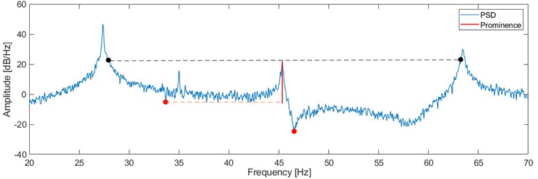
To determine proper values for block rows and model orders some information about the analyzed system must be acquired from the data. Namely this concerns the number and frequencies of the unknown eigenfrequencies. In the proposed algorithm this is done by examining the PSD of the data, where eigenfrequencies are visible due to their dominant visual appearance. The algorithm utilizes this to distinguish possible eigenfrequencies from noise influences by using the so-called ‘Prominence’, a parameter originating from Geography to describe the elevation of mountains relative to surrounding mountains. Some basic information and background can be found in [4]. This principle is shown in Fig. 2, where the prominence of a peak is basically its height above the lowest contour line that inherits the peak itself, but not a higher peak. It can be measured by drawing a horizontal line from any local maximum to both sides until the line either crosses the signal or reaches the start or end of the signal (black dashed line). On both sides covered by the horizontal line one can find a minimal value of the signal. The higher of both minima marks the relevant level (red dashed line) for the prominence of a peak. With this it is also clear that any noise peaks would have a vanishing prominence.

Fig. 2Exemplary prominence of a peak

Now, with the estimated $n$ eigenfrequencies $f_1,\dots ,f_n$ of the analyzed signal, one can set values for model order $k$ and block rows $i$ Eqs. (10-13):

where $i_{min}$ – minimal number of block rows, $i_{max}$ – maximal number of block rows, $k_{min}$ – minimal model order, $k_{max}$ – maximal model order.

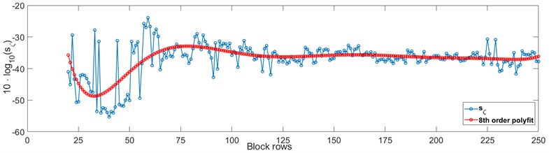
Since eigenfrequencies are estimated by calculating the eigenvalue decomposition, each eigenfrequency is represented by two (complex conjugated) eigenvalues, which leads to Eq. (12). The block Hankel matrix varies in size due to the iteration over the block rows Fig. 1. In this context Eq. (13) describes the maximum model order that can be calculated when using the smallest possible block Hankel matrix. Eq. (13) introduces a dependency on the number of sensors, which can be problematic, if a very large number of sensors is used. As described in [5], choosing a minimal number of block rows depends on the lowest frequency of interest and the sampling frequency. They proposed a rule of thumb similar to Eq. (10), but with an additional factor. This factor was herein omitted, which led to overall better results. To cover a large range of block rows, the corresponding maximal value is set by Eq. (11). The clustering of each stability plot is done via the hierarchical clustering method. This method has the advantage to work without any prior knowledge about the desired result, i.e. no number of clusters or their initial position must be provided. The applied criteria determine the characteristics of a cluster. In this context the criteria define the shape of an eigenfrequency in the plain of frequency and damping in the stability plot. In [6] a further description on hierarchical clustering is provided. First soft criteria are applied for the initial determination of clusters. The Modal Assurance Criterion (MAC) and a distance measure with respect to frequency and damping are used for this purpose. While the MAC compares the similarity of two mode-shapes and further details on this can be found in [7], the distance measure is shown in Fig. 3. Finally, hard validation criteria are used to eliminate physically meaningless poles and clusters. Therefore, poles with negative or very high damping (> 25 %), as well as very small cluster are omitted. The clustering yields a set of clustered stability plots. In the final step of the algorithm a sensitivity analysis w.r.t. the number of block rows is performed to find an optimal set of modal parameters. The basic idea is that with few block rows, the entire signal and noise contents are distributed over few singular values. With an increasing number of block rows, more singular values are rejected by model order reduction. Since the smallest singular values should contain mainly noise influences, this process improves the quality of the data for SSI-Cov. This is the decreasing part of the polyfit-approximation shown in Fig. 4 at around 25 block rows. With more block rows, the rejected singular values are no longer negligible small. In the corresponding part around 50 block rows the data quality is decreasing, since relevant signal information is cut out, too. With even more block rows this process reaches an equilibrium. For the sensitivity analysis this means that for every single stability plot with m clusters a mean standard deviation of the damping is calculated Eq. (14):

As described in [2], for the optimal choice of the number of block rows this value should have a minimum. An exemplary result for the sensitivity analysis is given in Fig. 4. The aforementioned trend to first decrease at relatively few block rows before increasing with more block rows is clearly visible. Outliers do appear at lower block rows, though the basic principle is still applicable.

Fig. 3Ellipse in plain of frequency and damping as distance measure

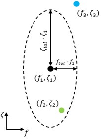
Fig. 4Sensitivity analysis criterium with polyfit approximation

4. Verification

The algorithm is validated on the example of a 3-DoF state space system. Additionally, three harmonic signals with 17 Hz, 40 Hz and 54 Hz respectively were added to the signal to simulate non-white noise excitation e.g. the influence of rotating machine parts, whose frequency can mirror into the calculation result. Table 1 provides the analytical parameters of the system.

Fig. 5 shows the stability plot for the conventional order reduction and the block row value that was found to be optimal by the sensitivity analysis. The stability plot for the modified order reduction is given in Fig. 6. Additional to the generally clearer appearance due to the more random distribution of mathematical poles, which is described in [1] in more detail, another important distinction between both methods can be made. The frequencies of the poles belonging to the added harmonics vary significantly more than those belonging to actual eigenfrequencies, when the modified method is used. For this system the iteration over the block rows ranged from 20 up to 200. As already indicated in Fig. 4, most times the optimum can be found at lower numbers of block rows. Accordingly, in this case the optimum was found at 40 block rows. As stated before, depending on the approach how the modified order reduction method is calculated, no sensitivity analysis is performed. This is the reason why there is only one result for the minimal number of block rows. Furthermore, as can be seen in both plots, the maximal order was set to 60. In a manual approach the model order would be set to a very high number to take the generally unknown real model order into account. Examining the PSD by using the Prominence parameter leads to a more reasonable value based on the actual system. This reduces the calculation effort considerably without losing quality of the result. In both stability plots, all three eigenfrequencies are clearly visible. Table 2 provides the corresponding calculation results. Comparing the modal parameters calculated with the two methods, the frequency estimates are almost equal. The damping estimates of the modified order reduction, however, differ more from the analytical results. This observation is based on the pre-SVD order reduction. At low model orders the Hankel matrix contains fewer system relevant information. A wider scattering around the analytical values of the corresponding modal parameters frequency and damping can be observed. The observation, that modal parameters calculated with the modified order reduction method show more variations around their analytical counterparts, especially the damping values (see. Table 2), should be the subject of further studies.

Fig. 5Stability plot for 3-DoF system with conventional order reduction and resulting eigenfrequencies (boxed)

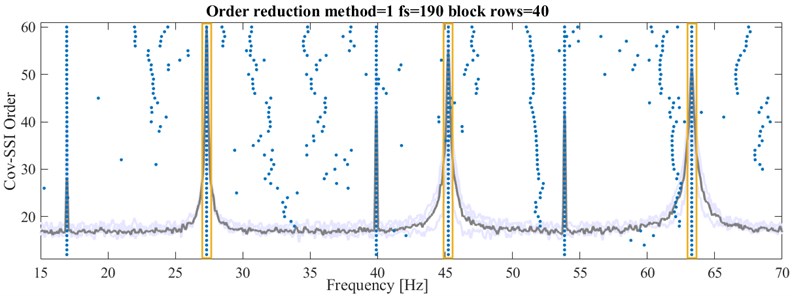
Fig. 6Stability plot for 3-DoF system with modified order reduction and resulting eigenfrequencies (boxed)

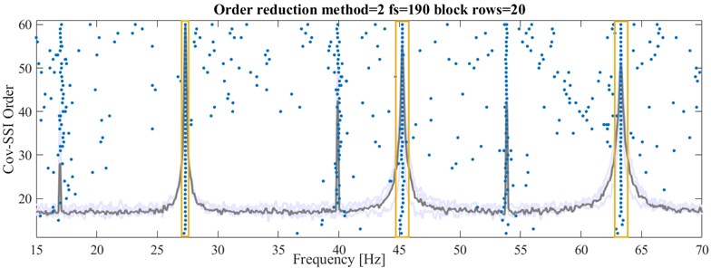
In both results none of the added harmonics is misinterpreted as an eigenfrequency, although at least Fig. 5 would visually allow for this mistake. In most results for different numbers of block rows, the added harmonic frequencies were found to be an eigenfrequency by the clustering. Therefore, with the damping criterion from Eq. (14), the sensitivity analysis was able to find the most optimal result.

5. Conclusions

The goal of this work was to develop an algorithm that allows a fully automated modal analysis. The first relevant step was the determination of input parameters. Using the prominence of a peak as a reference for its relevance, the algorithm mimics a visual interpretation of the PSD. In the example of chapter 4 the automatically determined input parameters led to good results. Further tests with more complicated systems have shown that especially weakly excited modes are hard to detect on this way. The averaged damping standard deviation as a criterion of the sensitivity analysis proved to locate the most optimal modal parameters in a set of results. If, however, some eigenfrequencies are not found by the peak-picking approach, the input parameters are not fitting for the actual system, which complicates the later analysis of the calculation results. One important step to improve the algorithm in future works is to improve the examination of the PSD to reliably analyze systems with weakly excited modes. Finally, the modified order reduction yielded good results with just the minimal number of block rows. As further tests have shown, the results of both order reduction methods converge to one another, if higher model orders are chosen for the modified method. This also indicates the necessity of further improvements in input parameter estimation, e.g. different approaches for both methods.

References

-
Wiemann Marcel, Bonekemper Lukas, Kraemer Peter Methods to enhance the automation of operational modal analysis. Vibroengineering Procedia, Vol. 31, 2020, p. 46-51.
Rainieri C., Fabbrocino G., Cosenza E. On damping experimental estimation. Proceedings of the 10th International Conference on Computational Structures Technology, 2010.
Rainieri C., Fabbrocino G. Operational Modal Analysis of Civil Engineering Structures. an Introduction and Guide for Applications. Springer, New York, 2014.
Kirmse A., De Ferranti J. Calculating the prominence and isolation of every mountain in the world, Progress in Physical Geography: Earth and Environment, Vol. 41, Issue 6, 2017, p. 788-802.
Reynders E., De Roeck G. Reference-based combined deterministic-stochastic subspace identification for experimental and operational modal analysis. Mechanical Systems and Signal Processing, Vol. 22, 2008, p. 617-637.
Murtagh F., Contreras P. Methods of Hierarchical Clustering. Computing Research Repository - CORR. 2011, arXiv:1105.0121.
Pastor M., Binda Harčarik M. T. Modal assurance criterion. Procedia Engineering, Vol. 48, 2012, p. 543-548.
About this article