Modal parameter identification of a three-storey structure using frequency domain techniques FDD and EFDD and time domain technique SSI: experimental studies and simulations

The aim of this study is to modal parameter identification of a three-storey structure using operational modal analysis. In this research, available techniques in both time domain and frequency domain have been utilized. In time domain, the Stochastic Subspace Identification (SSI) technique, and in the frequency domain, Frequency Domain Decomposition (FDD) and Extended Frequency Domain Decomposition (EFDD) have been used. The modal parameters of a three-storey structure have been calculated using both experimental and finite element method. For this purpose, first, the three-storey structure was modeled in the ANSYS software and then, using the vibration analysis, structural responses are determined. The structure responses are used as inputs of the operational modal analysis algorithms and the modal parameters are obtained. Then, by constructing and exciting the structure by a variety of external excitation, the responses are measured and then, they are used as inputs to the operational modal analysis algorithm to obtain the modal parameters. Since the input signal in OMA method should be random, random, periodic random, pseudo-random, and burst random signals are used for exciting the structure. Finally, the calculated modal parameters from the finite element method and empirical method are compared with each other.

1. Introduction

Dynamic analysis is one the most important and widely used engineering tools in designing, construction and maintenance of the structures, but usually there is no analytical solution for complex structures. Also, the approximate numerical methods like finite element, finite difference, and Differential Quadrature Method (DQM) have some problems such as errors resulting from the use of inappropriate assumptions, errors in modeling the details of complex structures and lack of information of the proper material properties. Therefore, the new techniques based on experiment are introduced as an appropriate tool for defining the dynamic properties of the structures.

Modal analysis is one the widely used methods in the industries, which is a technique for determining the intrinsic dynamic properties of a system including natural frequencies, damping factors, and mode shapes. Using these properties, a mathematical model of the dynamic behavior of the system can be proposed (modal model of the system), by which the designer could achieve a good insight for designing. Experimental modal analysis is in fact a procedure for the system identification. In the past two decades, numerous applications of modal analysis in the fields of engineering, science and technology have been reported. It is also expected that the application of the modal analysis grow rapidly in the future years [1]. Practical applications of the modal analysis have great relevance with the technological advances in the laboratorial methods. The reported applications of the modal analysis have been in the field of aeronautical engineering, structural and automobile engineering.

In Traditional Modal Analysis (TMA), the inputs and outputs of the system are measured, and then using the different methods of model identification such as peak picking and least square method, the modal parameters of the system are extracted. In general, the modal parameter identification of the system is done using the measured input and output data by Frequency Response Function (FRF) in the frequency domain or Impulse Response Function (IRF) in the time domain [2].

In recent years, researchers have been presented new methods of modal analysis based on measuring the response; so that by measuring the output response of the system regardless of input, the modal parameters could be found. These methods are named Operational Modal Analysis (OMA) or Output Only Modal Analysis (OOMA) [3]. The applied methods in the operational modal analysis are of the type of both time and frequency. Due to the accuracy of the obtained results, the available techniques in the time domain are superior to the existing techniques in the frequency domain. However, according to the less consumed time by the frequency techniques for finding the responses, such methods are also used.

The operational modal analysis is used in the large mechanical structures that the artificial excitation is impossible, and also in the structures being utilized, in which transferring to the laboratory environment is not possible. In these methods, the structure would not be excited using the traditional modal analysis method; rather the excitation is performed by the natural loadings. Since in this method, only the response is measured and the loading is unknown, the identification of the modal parameters should be conducted by the output data. As a result, special techniques are required for identifying the system with very small amplitude data without any information about the input force. In recent years, experimental methods for identification of the modal parameters have been widely used in the engineering applications.

Brincker et al. [4, 5] had proposed two nonparametric methods named Frequency Domain Decomposition (FDD) and Enhanced Frequency Domain Decomposition (EFDD), which have lots of similarity with complex mode identification and peak picking. They demonstrated that with the help of these two methods estimation of the modal parameters of the structure with good accuracy is feasible. First, they obtained the power spectral density matrix of the responses, and then determined the natural frequencies, damping coefficient and mode shapes by using the Singular Value Decomposition (SVD). Also, the effectiveness of these two methods is investigated on a two-storey structure with six-degree-of-freedom and assuming rigid motions of the floors. In the mentioned research, the model was excited with a white noise. Comparison of the obtained results from these methods with the theoretical results was indicated a close proximity of the results and insensitivity of the methods to the disturbance and external forces such as supports and environmental conditions. Also, the mode shapes obtained from these methods were similar to the theoretical ones.

Cuberg et al. [6] suggested a method applicable in both traditional and operational modal analysis. In this method, with the limited sampling data and calculating the Fourier spectra corresponding to the computed responses, the whole modal parameters of a structure could be achieved. They examined the validity of their methods for an aluminum plate with an acoustic excitation. Two methods were used by these researchers to gain the modal parameters. The first method was using the maximum probability estimator, which begins with FRF function. In the second method, a maximum estimator was used in the frequency domain. The excitation of the structure was conducted by two independent speakers. In one of the speakers, generating white noise would lead to excitation of the structure, and in the second one, the input electrical signal was measured as a system input.

The mode shapes obtained from OMA method, are un-scaled. For gaining the scaling factor, masses are added to specified points of the structures and the experiments are repeated. As a result of the change in the mass distribution, changes in the natural frequency of the structure are observed, from which the scaling factor would be achieved. Coppotelli [7] was studied the effects of different mass loadings on the plate and beam. In the first experiment, an aluminum cantilever beam with four-degree-of-freedom was subjected to a random excitation. The experiment was repeated four times and in each time, masses were added to the degrees of freedom. In the second experiment, a composite plate with free boundary conditions and 64-degree-of-freedom was used. In the second experiment as well as the first experiment, the experiment was repeated with the added masses. The results had indicated that the accuracy of the FDD and EFDD methods were high and they could be used as reliable methods in the engineering.

Zaghbani et al. [8] used the operational modal analysis as a powerful tool for determining the modal parameters of machine tool in the machining process. They analyzed data from the experiments by Least Square Complex Exponential Method (LSCE) and ARMA.

Zhang et al. [9] offered a new method for identification of the modal parameters of a structure, named frequency-spatial domain decomposition. They revealed that the modal identification functions could be achieved from the eigenvalue plots resulted from the power spectral density matrix. Also, the mode shapes can be determined directly from eigenvectors corresponding to the eigenvalues in the peak of the modal identification functions diagrams. The damping coefficients and natural frequencies of the system were specified from curve fitting on the power spectral density matrix. Although this method is considered as a narrow-band identification process and is able to identify a single mode at any time, but it can be used for the structures with modes very close to each other.

Allen et al. [10] suggested a method for identifying the modal parameters of linear and periodically time-varying system, where the exciting force is not measurable, random and with a broad band. They checked their method by determining the modal parameters of a wind turbine.

Mohanti et al. [11] offered a method that estimates the modal parameters with great accuracy in the case of existing a harmonic component in the system response (for example, due to the presence of the rotating component). If the frequency of the harmonic parts is close to the particular frequencies of the system, the operational modal analysis would not be able to identify the parameters, exactly. Therefore, the implemented the proposed method known as the least square complex exponential identification procedure on the beam, in which in addition to random excitations, harmonic loadings were exerted.

Huang et al. [12] proposed Hilbert-Huang transform method for signal processing. The advantages of this method compared to the previous methods in signal processing were the capability of processing all signals including linear and nonlinear, and also stationary and non-stationary signals. This method compromises empirical mode decomposition and Hilbert transform. In the first part, the empirical mode decomposition is applied on the initial signal, which decomposes the signal to a set of simple signals, named intrinsic mode decomposition. In the second part, the Hilbert transformation would be applied on the intrinsic mode decomposition.

Hera et al. [13] investigated the variations in the natural frequencies and mode shapes in order to evaluate the health structure evaluation. In their investigation, for identifying the defects in the structure three methods of continuous wavelet transform, empirical mode decomposition, and wavelet pocket were employed. They modeled a system of mass-spring-damper with three-degree-of-freedom, and created two sudden and gradual defects on it. Comparison between the aforementioned methods indicated that the all methods are able to identify the gradual defect. In the case of sudden defect, wavelet pocket method showed better performance compared to other methods. In the presence of disturbance in the obtained data, continuous wavelet transform was superior. The accuracy of the continuous wavelet transform and wavelet pocket method is highly dependent on the selected mother wavelet function. If the mother wavelet function is selected inappropriately, satisfactory results from these methods would not be achieved, however in the empirical mode decomposition this deficiency does not exist, because no pre-defined function (to approximate the signal) is used.

Gao et al. [14] investigated the fault cause in a rotary machinery using empirical mode decomposition method. They also aimed to improve this method. They used combined mode function rather than intrinsic mode decomposition. The combined mode function is a combination of adjacent intrinsic modes. In their study, the system was a high pressure cylinder of power generator that had one broken bearings. The cause of breaking was investigated by empirical mode decomposition and using combined mode function. Finally, the friction between the bearing and rotor, and simultaneously, the impact exerted on the bearing was demonstrated as the main cause of break in the bearing. In addition, comparing the results of empirical mode decomposition method and wavelet analysis, better results were observed in identifying the crack by the empirical mode decomposition method.

Tarinejad et al. [15] calculated the modal parameters of three-degree-of-freedom system by combining the FDD and wavelet transform methods. They first modeled the system with random excitation in the MATLAB/Simulink software and obtained the time response. Then, by eliminating the disturbance from the time response, the natural frequencies and mode shapes were calculated by FDD method. Finally, the damping coefficient of the model was determined by wavelet transformation.

Ebrahimi et al. [16] computed the natural frequencies of a cutting blade of Harvesters using FDD method and actual data (during operation). In addition, the blade was modeled in the ANSYS software and considering the relative difference between the natural frequencies, the model was corrected and an accurate model of the system was created in the software. The resonance was prevented by adding the point masses to the blade.

Ventura et al. [17] studied the vibration of Wilshire tower in California by installing 20 accelerometers in different directions. After 4 years, an earthquake occurred in the distance of 30 kilometers from California, although this earthquake was lasted a few seconds, but was lead to a displacement in the structure for about three minutes. They calculated the natural frequencies, damping coefficient and mode shapes of the structure by operational modal analysis and FDD method using ARTeMIS software.

Guo et al. [18] introduced a new method for identification of the damping coefficient of the linear systems in the frequency domain by integral method. In their survey, first the FRF diagram was transformed to other types of frequency dependent diagrams. Then by integrating the area under the diagram, the damping coefficients were calculated. They introduced three FDI-1, FDI-2 and FDI-3 methods, among which the FDI-3 method was proposed due to the higher accuracy and simple algorithm.

Stochastic Subspace Identification (SSI) proposed by Overschee et al. [19], is a developed method that have been proposed as an alternative to the traditional methods. In this method, the state space is calculated from measurements of the system output.

Kompala et al. [20] compared the data from finite element method with the data from empirical modeling in order to investigate the accuracy of the identification algorithms in the stochastic subspace in determining the damage and its location. For creating crack, they used a special tool in the cantilever beam and obtained the system responses and then, imported them into the stochastic subspace algorithms. They demonstrated that the stochastic subspace algorithms are able to predict the presence of the damage and its location with a good accuracy by the direct use of the data.

Noel et al. [21] developed a new method by combining the stochastic subspace with frequency methods for calculating the modal parameters of nonlinear systems. To verify the method, the modal parameters of a five-degree-of-freedom system with two nonlinear components (two non-linear springs) were calculated. Also, they devised a new method, named time-domain nonlinear subspace identification by adding a nonlinear component to the SSI method. They used this method for defining the dynamic parameters of EADS spacecraft

Gorsat et al. [22] analyzed the vibrational data from a spacecraft. According to the complexity of the vehicle and many different parts used in the structure, determining the modal parameters of the vehicle was faced with many challenges. The modal analysis of the structure was performed by stochastic subspace algorithms with two methods of data driven and calculation of the covariance functions. It was demonstrated that the natural frequencies change in small amounts, however, the mode shapes are more stable. In addition, despite the closeness of the results from both methods, the damping coefficients obtained from covariance functions are more accurate.

In this research, modal parameters of a three-storey structure have been calculated using both experimental and finite element method. The structure responses are used as inputs of the operational modal analysis algorithms and the modal parameters are obtained. Finally, the calculated modal parameters from the finite element method and empirical method are compared with each other.

2. Operational modal analysis method in the frequency domain

2.1. FDD technique

The Frequency Domain Decomposition (FDD) is one of the nonparametric operational modal analysis in the frequency domain which have lots of similarity with complex mode identification and peak picking. It is assumed the structure is excited by a signal with a wide frequency band having the same amplitude in all frequencies (white noise). According to the made assumption in relation to the input excitation type, the structural analysis is performed only on the basis of the output data.

Assuming that the number of accelerator in the structure is $m$ , the response vector of the system would be an $m \times 1$ vector. It is also assumed that the white noise is applied on the $k$ th points of the stricter, so the input is a $k \times 1$ vector [4, 5]. The spectral density function is an $m \times m$ matrix as below:

1

G_{y y} (j ω) = H (j ω) G_{x x} (j ω) H^{H} (j ω), - \infty < ω < \infty .

In the above equation, $G_{x x} (j ω)$ and $G_{y y} (j ω)$ are the spectral density function of the input and output. Also, $H (j ω)$ is an $m \times k$ frequency response function matrix, which represents the relation between the input and the output. The Superscript $H$ is the indicator of Hermitian transformation (complex conjugating and then transposing). The importance of the spectral density function is that the natural frequencies of system are recognizable as the peaks in the spectral density function diagram. Assuming the white noise excitation, the $G_{x x} = C$ matrix would be a constant matrix with real and symmetric values.

Assuming that the spectral density function $G_{y y} (j ω)$ is estimated in the distinct frequencies of $ω = ω_{j} \geq 0$ , the function would be determined by a series of spectral density matrixes corresponding to a distinct frequency as following [4, 5]:

2

G_{y y} (j ω) = [\begin{matrix} {\bar{Y}}_{1} (j ω) {\bar{Y}}_{1} (j ω) & {\bar{Y}}_{1} (j ω) {\bar{Y}}_{2} (j ω) & \dots & {\bar{Y}}_{1} (j ω) {\bar{Y}}_{r} (j ω) \\ {\bar{Y}}_{2} (j ω) {\bar{Y}}_{1} (j ω) & {\bar{Y}}_{2} (j ω) {\bar{Y}}_{2} (j ω) & \dots & {\bar{Y}}_{2} (j ω) {\bar{Y}}_{r} (j ω) \\ ⋮ & ⋮ & ⋱ & ⋮ \\ {\bar{Y}}_{m} (j ω) {\bar{Y}}_{1} (j ω) & {\bar{Y}}_{m} (j ω) {\bar{Y}}_{2} (j ω) & \dots & {\bar{Y}}_{m} (j ω) {\bar{Y}}_{r} (j ω) \end{matrix}],

where, ${\bar{Y}}_{r} (j ω)$ corresponds to the $r$ th frequency. Using the SVD method, the spectral density function is decomposed as below:

3

G_{y y} (j ω) = U_{j} S_{j} V_{j}^{H} = u_{j 1} s_{j 1} v_{j 1}^{H} + u_{j 2} s_{j 2} v_{j 2}^{H} + \dots + u_{j m} s_{j m} v_{j m}^{H} .

In the above relation, $U_{j}$ and $V_{j}$ are the unique matrixes that the columns represent the orthogonal eigenvectors $G_{y y} (j ω)$ in the $ω = ω_{j} \geq 0$ frequencies. We have:

4

U_{j} = [u_{j 1}, u_{j 2}, \dots, u_{j m}], V_{j} = [v_{j 1}, v_{j 2}, \dots, v_{j m}], U_{j} = V_{j},

where, $S_{j}$ is the diagonal eigenvalues matrix of $G_{y y} (j ω)$ . By approaching the $ω$ to the modal frequency, the output PSD matrix would be transformed to a first order matrix according to the following relation [4, 5]:

5

G_{y y} (j ω) = u_{j} s_{j} v_{j}^{H} .

In this case, the first column of matrix $U$ is approximation of normalized mode shape vector. One of the properties of the SVD method is that the eigenvalues and corresponding eigenvectors are placed in a descending manner in the matrix. The first eigenvector of matrix $u_{j 1}$ would be an estimation of the mode shapes. In the other words, by determining the eigenvalue in the peak, the first corresponding eigenvector would be an approximation of mode shape vector. By moving away from the peak, the effects of other eigenvalues become apparent.

As mentioned above, for an acceptable approximation of the mode shapes, it can be relied on the corresponding mode shapes to the natural frequencies, which are equivalent to the first column of matrix $U$ . however, for an accurate expression of the mode shapes, vectors similar to the desired mode shape can be recognized, by averaging these vectors, more accurate approximation of the mode shapes would be presented. For this purpose, first a peak should be specified, and then, the corresponding eigenvector would be determined. Afterwards, the vectors resembling the eigenvector would be searched in the vicinity of the peak, using MAC method. The MAC method is given as follows [4, 5]:

6

M A C (i, j) = \frac{{|ϕ_{i}^{T} ϕ_{j}|}^{2}}{|ϕ_{i}^{T} ϕ_{i}| |ϕ_{j}^{T} ϕ_{j}|},

where, $ϕ_{i}$ is the corresponding mode shape with dominant frequency (peak) and $ϕ_{j}$ is the corresponding mode shape with frequencies in the vicinity of the peak. The MAC index represents the cosine of the angle between the mode shape vectors. If the mode shape vectors are coincident, the index would be equal to 1, and for two orthogonal vectors, it would be 0. In different references, the values between 0.85 and 1 are acceptable for MAC criteria [4, 5].

2.2. EFDD technique

The exact damping coefficients of the system could not be achieved with FDD technique [4, 5]. Therefore, a developed method, EFDD, is proposed. The natural frequencies and damping coefficient for each mode can be obtained from this method. After calculating the power spectral density matrix of the system response and SVD analysis on the response, the response function using the inverse Fourier transformation is transformed from the frequency domain to the time domain. The resulting function is named correlation function [4, 5]. Using the correlation function, the natural frequencies and damping coefficients can be achieved by crossing time approximation and logarithmic decrement. For this purpose, specific area of the correlation function (the area specified in Fig. 1) is considered. Near the beginning and end of the diagram, the function is subjected to the possible disturbance and nonlinear effects of the structure, which would lead to an error in the identification of the system parameters, so, these parts are not considered. Then, the extremum of the correlation diagram would be determined [4, 5].

Fig. 1The correlation function

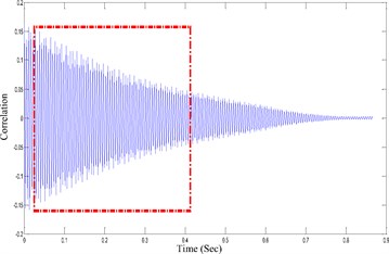
Modal parameters of the system can be obtained from the logarithmic decrement [4, 5]:

7

δ = \frac{1}{n} l n |\frac{x_{1}}{x_{n + 1}}| = \frac{2 π ζ}{\sqrt{1 - ζ^{2}}} .

In the above relation, $δ$ is the logarithmic decrement, $ζ$ is the damping ratio, $x_{1}$ is the amplitude in the beginning of the correlation function diagram, and $x_{n + 1}$ is the amplitude after $n$ cycles. Also, the natural frequency of the system can be obtained by creating a linear regression on the crossing time and the times corresponding to the extremum values [4, 5].

2.3. The SSI operational modal analysis in the time domain

The subspace identification methods can be used in the cases where the input signal is deterministic, random, or combination of them. The SSI method is used for identification of the modal parameters with the random input signal. As well as the FDD method, the inputs are unknown in the SSI method. In this method, white noise with Gaussian distribution and zero mean is used [19], and there is no need for using FFT to transform the signal from the time domain to the frequency domain and the data in the time domain are utilized directly. This property eliminates the leakage error in the data and the variation in the stiffness matrix due to the use of windowing function. It should be mentioned that the existing algorithms in the time domain require large amounts of measurement data, and therefore, these methods are very time-consuming.

The equation motion of an $n$ -degree-of-freedom linear discrete system with constant parameters and viscous damping subjected to the white noise is as follows:

8

\begin{array}{l} x (k + 1) = A_{d} x (k) + B_{d} w (k), \\ y (k) = C x (k) + v (k), \end{array}

where, $x (k)$ is the state vector, $y (k)$ is the output vector, and $v (k)$ is the disturbance due to the measurement, which implies the difference between the state variables and measured outputs. Also, $w (k)$ is a random excitation as an input, which is a noise caused by processing. Both the disturbances due to the measurement and processing are of the type of white noise with Gaussian distribution and zero mean [19]. In this method, the covariance of the output signals $y (k)$ is used to identification of the modal parameters of the system. Here, the variables of the covariance are considered $p$ and $q \leq p + 1$ . Higher values for $p$ provide better evaluation of results. Generally, $q = p - 1$ is selected. The Henckel matrix would be constructed from the response function covariance. We have [19, 22]:

9

H_{p + 1, q} = [\begin{matrix} R_{1} & R_{2} & \dots & R_{q} \\ R_{2} & R_{3} & \dots & R_{1 + q} \\ ⋮ & ⋮ & ⋱ & ⋮ \\ R_{p + 1} & R_{p + 2} & \dots & R_{p + q} \end{matrix}] .

In which, $H$ is the Henkel matrix and $R$ is the covariance of the response function. The Henkel matrix is decomposed to controllability matrix and observability matrix through the RQ decomposition method. We have:

10

H_{p + 1, q} = O_{p + 1} χ_{q}

where, $O_{p + 1}$ is the observability matrix and $χ_{q}$ is the controllability matrix. Using the SVD method:

11

H_{p + 1, q} = U Δ V^{T} = (U_{1} U_{0}) (\begin{array}{l} Δ_{1} 0 \\ 0 Δ_{0} \end{array}) V^{T}, O_{p + 1} = U_{1} Δ_{1}^{1 / 2} .

Matrix $H$ , which has an important role in identification of the modal parameters of a system, is equal to the first block-row of the observability matrix $O_{p + 1}$ (see the Eq. (12)). The state-transition matrix $F$ , would be achieved from the shift invariance property of $O_{p + 1}$ matrix [20, 23]:

12

O_{p + 1} (H, F) = (\begin{matrix} H \\ H F \\ ⋮ \\ H F^{p - 1} \end{matrix}), O_{p}^{↑} (H, F) = O_{p + 1} (H, F) F .

For obtaining the $F$ matrix, assuming $r a n k (O_{p}) = d i m F$ is required. Thus, that the number $p + 1$ of block-rows in $H_{p + 1, q}$ is large enough. The eigenvalues and eigenvectors of the system can be determined from matrix $F$ . We have:

13

d e t (F - λ I) = 0, F φ_{λ} = λ φ_{λ} .

In which, $λ$ is the eigenvalue, and $φ_{λ}$ is the eigenvector of the $F$ matrix. Consequently, the natural frequencies, damping ratios and mode shapes of the system can be determined. The natural frequencies $(ω_{f})$ and damping ratios $(ζ)$ are calculated as following:

14

\begin{matrix} a = |a r c t a n (\frac{I m λ}{R e λ})|, b = l n |λ|, ω_{f} = \frac{a}{2 π τ}, ζ = \frac{100 |b|}{\sqrt{a^{2} + b^{2}}} . \end{matrix}

Also, the mode shapes $(ϕ_{λ})$ are specified as:

15

ϕ_{λ} = H φ_{λ} .

3. The structure and testing equipment

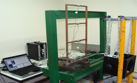
The desired three-storey structure is composed from two vertical beams with the length of 65 cm and three horizontal beams with the length of 30 cm. The horizontal beams are connected to the vertical beams, at equal distances and by welding. Additionally, the vertical beams are connected to a steel part as a support. The cross section of the beam and the used steel is the same in the whole structure. The desired structure and testing equipment are indicated in Fig. 2.

Fig. 2The desired structure and testing equipment

The structure is excited using an electrodynamics shaker. When the output electrical current from the signal generator passes through the coil of the shaker, a force proportional to the electrical current and magnetic flux density is generated, which moves the drive rod. The shaker is connected to the main structure by a connecting rod named stinger (see Fig. 3). Stinger is a rod that its geometry is selected in a way that minimizes the flexural stiffness and maximizes the axial stiffness. The main purpose of using stinger is dynamic separation of the shaker from the structure; however, it would not have achieved completely. The connecting location of the shaker is placed on the support, which reduce the dynamic effects of the shaker on the system responses.

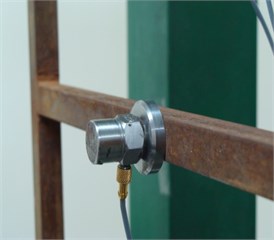
Five accelerometers are used for measuring the responses of the structure. These accelerometers are connected to the structure by magnet (see Fig. 4).

Fig. 3The electrodynamics shaker and stinger

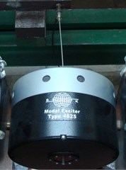
Fig. 4The connection of the accelerometer to the structure

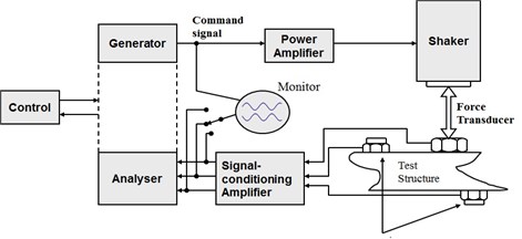
In Fig. 5, the schematic diagram of the measuring and processing system, including: signal generator, shaker, excretion of the force, measuring the response and signal processor, is presented.

Fig. 5The measuring and processing system

4. FEM modeling

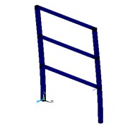
The three-storey structure is modeled in the ANSYS software, and then, by vibrational analysis, the acceleration responses are obtained. The structure responses are imported as input to the operational modal analysis methods algorithm, and the modal parameters of the structure are determined. For modeling the structure in the ANSYS, the Solid 186 elements are used due to the three-dimensional modeling of the structure, also, this element is able to indicate the flexural and torsional modes. The model of the structure in the ANSYS software is presented in Fig. 6.

The vertical beams are welded to a rigid rod from the bottom end. This solid rod is limited the motion of the vertical beams in x, y, and z direction and restricts the rotation of the structure. The stinger causes an additional stiffness in the system, which would lead to a change in the frequencies of the structure. Consequently, the best method for modeling the stinger is using a linear spring. The combination 14 elements are used for modeling the linear spring. This element is capable of modeling the spring and damped. An overview of the structure, including physical model, supports and linear spring is shown in Fig. 6.

Fig. 6The model of the three-storey structure in the ANSYS software

4.1. Validation of the FEM model

Prior to loading the structure model in the ANSYS software, the accuracy and validity of the FEM method should be ensured. For this purpose, the natural frequencies of the system are calculated from FEM method and traditional modal analysis, and the results are compared with each other. The modal analysis is used for determining the natural frequencies of the structure in the ANSYS software. This analysis is able to calculate the modal parameters, including natural frequencies and mode shapes of the system. For determining the natural frequencies from the TMA methods, the structure is excited by hammer (Global Test Type AU02). The response is measured by an accelerometer (DJB Type). The output signal of the accelerometer is transferred to the signal analyzer (B&K Type 3032A), and finally the FFT would be performed on the time response. The system response is observed with the help of the pulse software. Eventually, the frequency response and the model is imported to the MeScope software, and the natural frequencies, mode shapes and damping coefficients are computed from the frequency diagram. In Table 1, the natural frequencies of the structure, finite element model and traditional modal analysis method, are compared.

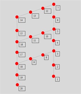
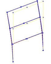
In Fig. 7, the structure model is presented in the MeScope software. The marked colored points represent the location of hammer impacts.

Table 1The natural frequencies of the structure (Hz), FEM and TMA

Method	First	Second	Third	Fourth	Fifth	Sixth	Seventh
FEM	15.60	55.02	93.40	167.70	243.44	373.89	404.90
TMA	15.44	54.76	93.13	168.24	245.12	378.52	413.37

Fig. 7The structure model in the MeScope software

In Fig. 8, the diagram of the relative error percentage of the FEM method compared with the traditional modal analysis is presented.

According to the Fig. 8, the percentage of the relative error in the natural frequency is acceptable; the highest error is due to the seventh frequency with the value of 2.05 percentages. So, the FEM model is verified. In Fig. 9, the first five modes of the structure by FEM method is indicated.

Fig. 8The diagram of the relative error percentage of the FEM method compared with the TMA

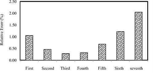
Fig. 9The first five modes of the structure according to the ANSYS software

a) First mode shape

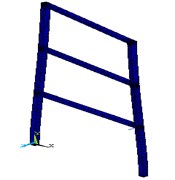
b) Second mode Shape

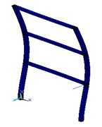
c) Third mode shape

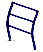
d) Fourth mode Shape

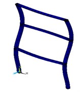
e) Fifth mode Shape

4.2. Calculating the modal parameters

As it was noted before, the excitation of the structure is conducted by a shaker, where the output is a random displacement. The transient solution is used for modeling the excitation of the structure. To this end, a random input with the amplitude of 5 mm is applied on the structure, after 5000 times of oscillation, the acceleration responses are measured in the nodes. It should be noted that the spring is allowed to move in the $z$ direction. The possibility of measuring the acceleration in all of the structure nodes is one of the transient solution characteristics in ANSYS software. As a result, each node in the finite element model of the structure is the representative of an accelerometer. Finally, the acceleration response of some nodes is selected as inputs to the SSI, FDD, and EFDD algorithms and the modal parameters of the structure would be determined.

In Fig. 10, the power spectral density of the system response by FDD algorithm is presented. The peak points of the power spectral density are the natural frequencies of the system.

In Fig. 11, the stabilization diagram of the structure for calculating the natural frequencies by SSI method is plotted.

In Fig. 12, the percentage of the relative error in the natural frequencies of the SSI, FDD and EFDD methods compared to the FEM method is presented.

In Table 2, the natural frequencies of the structure are provided by SSI, FDD and EFDD methods.

Fig. 10The diagram of power spectral density of the system response, FEM model (FDD method)

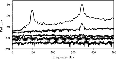
Fig. 11The stabilization diagram of the structure for calculating the natural frequencies (Hz), SSI method

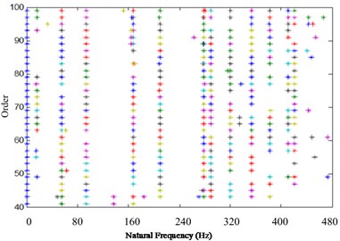
Fig. 12The percentage of the relative error in the natural frequencies of the SSI, FDD and EFDD methods compared to the FEM method

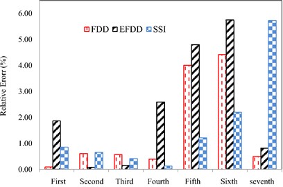
Table 2The natural frequencies of the structure (Hz), FEM model (SSI, FDD and EFDD methods)

Method	First	Second	Third	Fourth	Fifth	Sixth	Seventh
FDD	15.62	54.68	92.86	167.02	253.21	357.37	402.87
EFDD	15.90	54.97	93.54	163.34	255.15	352.40	401.58
SSI	15.74	54.66	91.42	167.48	246.41	365.68	428.09

Fig. 13The first three modes obtained from the SSI and FDD methods, the solid line is the indicator of mode shapes by SSI method, and the dashed line is for FDD method

The first three modes obtained from the SSI and FDD methods, the solid line is the indicator of mode shapes by SSI method, and the dashed line is for FDD method

a) First mode shape

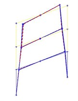
b) Second mode shape

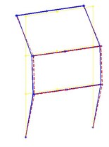
c) Third mode shape

According to the figure, the highest error value is related to the sixth mode in the EFDD method, and seventh mode in the SSI method (about 6 %). In Fig. 13, the first three modes obtained from the SSI and FDD methods are plotted. As it mentioned in previous sections, EFDD is unable to determine the mode shapes. The solid line is the indicator of mode shapes by SSI method, and the dashed line is for FDD method.

5. Experiment

The structure and testing equipment, also measuring and processing system are shown in Figs. 2 and 5, respectively. The shaker is able to generate different kinds of signals. Since the input signal in the OMA methods should be random, so only the random, periodic random, pseudo-random and burst random are used for excitation. The signals are filtered through a low-pass filter with the cutoff frequency of 1600 Hz and then transmitted to the shaker. The shaker excites the structure for about 10 seconds, the time signals corresponding to the responses are measured for 10 seconds and with the sampling frequency of 16384 Hz.

The response signals are imported to the OMA algorithms without being filtered. The aliasing problem is prevented due to the provided consideration. In Fig. 14, the values of the SVD on a spectral density data (burst random excitation) are presented.

In Table 3, the natural frequencies of the structure obtained from the experiments by FDD method is provided.

Fig. 14The values of the SVD on a spectral density data (burst random excitation), FDD

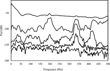
Table 3The natural frequencies of the structure obtained from the experiments (FDD method) (Hz)

Signal	First	Second	Third	Fourth	Fifth	Sixth	Seventh
Random	14.22	54.00	89.50	165.72	244.98	367.04	403.66
Pseudo-random	13.72	52.73	91.01	166.98	248.14	368.80	404.61
Burst random	13.04	50.89	87.39	165.00	244.86	369.47	407.64
Periodic random	13.40	51.65	88.71	166.17	246.32	363.86	399.83

Table 4The natural frequencies of the structure obtained from the experiments (EFDD method) (Hz)

Signal	First	Second	Third	Fourth	Fifth	Sixth	Seventh
Random	15.90	51.46	88.09	166.96	249.10	372.62	403.72
Pseudo-Random	16.60	49.74	86.53	165.14	242.83	369.20	405.24
Burst Random	13.04	59.90	85.28	167.44	244.49	375.27	410.09
Periodic Random	13.37	51.89	84.72	166.06	251.74	370.61	403.04

Table 5The natural frequencies of the structure obtained from the experiments (SSI method) (Hz)

Signal	First	Second	Third	Fourth	Fifth	Sixth	Seventh
Random	15.47	51.46	85.87	167.78	246.27	376.28	408.11
Pseudo-Random	15.61	49.74	87.80	163.53	245.31	372.33	407.62
Burst Random	14.85	59.90	90.43	165.41	244.82	373.82	408.93
Periodic Random	15.13	51.89	90.62	162.93	244.32	371.82	410.37

In Table 4, the natural frequencies of the structure obtained from the experiments by EFDD method is provided.

In Table 5, the natural frequencies of the structure obtained from the experiments by SSI method is provided.

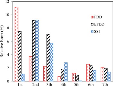
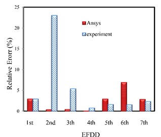
In Fig. 15, the percentage of the relative error of the natural frequencies resulted from the experiments using SSI, FDD and EFDD methods are indicated compared to TMA (Table 1). The higher frequencies are more accurate, so the maximum error percentage is related to FDD method for random excitation.

In Fig. 16, the percentage of the relative error of the natural frequencies resulted from the experiments using SSI, FDD and EFDD methods are indicated compared to TMA for pseudo-random excitation. The highest error is observed in the first three signals and also SSI method shows more accurate results.

Fig. 15The percentage of the relative error of the natural frequencies resulted from the experiments using SSI, FDD and EFDD methods compared to TMA for random excitation

The percentage of the relative error of the natural frequencies resulted from the experiments using SSI, FDD and EFDD methods compared to TMA for random excitation

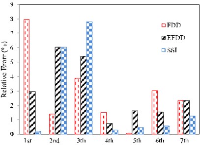
Fig. 16The percentage of the relative error of the natural frequencies resulted from the experiments using SSI, FDD and EFDD methods compared to TMA for pseudo-random excitation

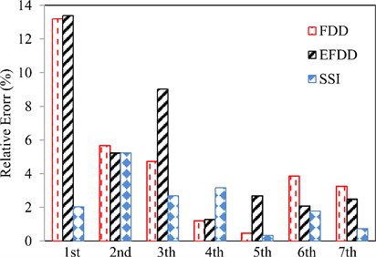
In Fig. 17, the percentage of the relative error of the natural frequencies resulted from the experiments using SSI, FDD and EFDD methods are indicated compared to TMA for burst random excitation. Higher frequencies show more accurate results compared to lower frequencies.

In Fig. 18, the percentage of the relative error of the natural frequencies resulted from the experiments using SSI, FDD and EFDD methods are indicated compared to TMA for periodic random excitation.

Fig. 17The percentage of the relative error of the natural frequencies resulted from the experiments using SSI, FDD and EFDD methods compared to TMA for burst random excitation

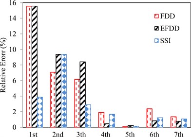
Fig. 18The percentage of the relative error of the natural frequencies resulted from the experiments using SSI, FDD and EFDD methods compared to TMA for periodic random excitation

For investigating the effect of different excitation signals on the natural frequencies of the structure, in Fig. 19, the percentage of the relative error of the natural frequencies resulted from the experiments using SSI, FDD and EFDD methods are indicated compared to TMA for four random excitations. The SSI shows lower error, and also, the frequencies obtained from the random method, indicate more appropriate adaptation to the traditional method results.

In Tables 6 and 7, the damping coefficients resulted from the experiment by SSI and EFDD methods are provided for four excitement signals. The FDD is not able to compute the damping coefficients.

Fig. 19The percentage of the relative error of the natural frequencies resulted from the experiments using SSI, FDD and EFDD methods compared to TMA for four random excitations

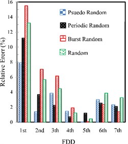
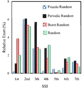
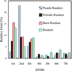
Table 6Damping coefficients resulted from the experiment by EFDD methods for four excitement signals

Signal	First	Second	Third
Random	2.59	0.28	0.78
Pseudo random	1.39	0.27	1.41
Burst random	1.98	0.33	1.21
Periodic random	2.91	0.21	1.12

Table 7Damping coefficients resulted from the experiment by SSI methods for four excitement signals

Signal	First	Second	Third
Random	1.31	0.40	0.71
Pseudo random	2.61	0.39	1.22
Burst random	1.37	0.41	1.55
Periodic random	3.71	0.22	1.39

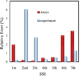
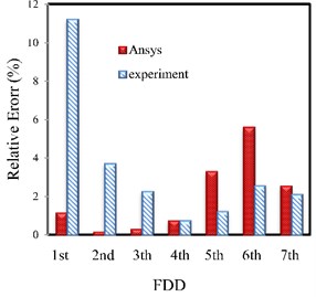
In Fig. 20, the relative error percentage of the natural frequencies resulted from the experiments using SSI, FDD and EFDD and FEM (ANSYS) methods are indicated compared to TMA for random excitation. As it mentioned earlier, the computed frequencies using the random excitation signals gain the least error compared to TMA.

According to the figure, the frequency adaptation is better in SSI method than the other two methods. Also, in the lower frequencies, the FEM method, and in higher frequencies, the OMA represent lower error percentage compared to TMA. The reason is due to the inability of the OMA in recognizing the lower frequencies of the system with high accuracy.

Fig. 20The relative error percentage of the natural frequencies resulted from the experiments using SSI, FDD and EFDD and FEM (ANSYS) methods compared to traditional modal analysis for Random excitation

The relative error percentage of the natural frequencies resulted from the experiments using SSI, FDD and EFDD and FEM (ANSYS) methods compared to traditional modal analysis for Random excitation

6. Conclusions

The modal parameters of a three-storey structure identified using the operational modal analysis (OMA), both experiments and FEM. The modal parameters of a three-storey structure calculated using both experimental and finite element method (FEM). At first, the three-storey structure modeled in the ANSYS software and then, using the vibration analysis, structural responses determined. The structure responses are used as inputs of the OMA algorithms and the modal parameters obtained. Then, by constructing and exciting the structure by a variety of external excitation, the responses measured and they are used as inputs to the OMA algorithm to obtain the modal parameters. Finally, the calculated modal parameters from the FEM and empirical method compared with each other.

The percentage of the relative error of the natural frequencies resulted from the experiments using SSI, FDD and EFDD methods compared to TMA. For investigating the effect of different excitation signals on the natural frequencies of the structure, the percentage of the relative error of the natural frequencies resulted from the experiments using SSI, FDD and EFDD methods compared to TMA for four random excitations (random, periodic random, pseudo-random, and burst random). The SSI shows lower error, and also, the frequencies obtained from the random method, indicate more appropriate adaptation to the TMA results. The percentage of the relative error of the natural frequencies resulted from the experiments using SSI, FDD and EFDD methods compared to TMA for periodic random excitation. Also, the percentage of the relative error of the natural frequencies resulted from the experiments using SSI, FDD and EFDD methods compared to TMA for pseudo-random excitation. The highest error observed in the first three signals and also SSI method shows more accurate results. The relative error percentage of the natural frequencies resulted from the experiments using SSI, FDD and EFDD and FEM (ANSYS) methods compared to TMA for random excitation. The computed frequencies using the random excitation signals gain the least error compared to TMA. The frequency adaptation is better in SSI method than the other two methods. For the design of real bodies or structures to dynamic actions it is better to use SSI method. Also, in the lower frequencies, the FEM method, and in higher frequencies, the OMA represent lower error percentage compared to TMA.

References

Fu Z. F., He J. Modal Analysis. Butterworth-Heinemann, First Edition, United Kingdom, 2001.

Search CrossRef
Ewins D. J. Modal Testing: Theory, Practice and Application. Research Studies Press, United Kingdom, 2000.

Search CrossRef
Zhang Y., Zhang Z., Xu X., Hua H. Modal parameter identification using response data only. Journal of Sound and Vibration, Vol. 282, Issues 1-2, 2005, p. 367-380.

Publisher
Brincker R., Andersen P., Zhang L. Modal identification from ambient responses using frequency domain decomposition. Proceedings of the 18th International Modal Analysis Conference (IMAC), San Antonio, Texas, 2000, p. 625-630.

Search CrossRef
Brincker R., Ventura C. E., Andersen P. Damping estimation by frequency domain decomposition. Proceedings of the 19th International Modal Analysis Conference (IMAC), Kissimmee, Florida, 2001, p. 698-703.

Search CrossRef
Cauberghe B., Guillaume P., Verboven P., Parloo E. Identification of modal parameters including unmeasured forces and transient effects. Journal of Sound and Vibration, Vol. 265, Issue 3, 2003, p. 609-625.

Publisher
Coppotelli G. On the Estimate of the FRFs from operational. Mechanical Systems and Signal Processing, Vol. 23, Issue 2, 2009, p. 288-299.

Publisher
Zaghbani I., Songmene V. Estimation of machine-tool dynamic parameters during machining operational trough operational modal analysis. International Journal of Machine Tools and Manufacture, Vol. 49, Issue 12, 2009, p. 947-957.

Publisher
Zhang L., Wang T., Tamura Y. A frequency-spatial domain decomposition (FSDD) method for operational modal analysis. Mechanical Systems and Signal Processing, Vol. 24, Issue 5, 2010, p. 1227-1239.

Publisher
Allen M. S., Sarcic M. W., Chauhan S., Hansen M. H. Output-Only modal analysis of linear time-periodic system with application to wind turbine simulation data. Mechanical Systems and Signal Processing. Vol. 25, Issue 4, 2011, p. 1174-1191.

Publisher
Mohanty P., Rixen D. J. Operational modal analysis in the presence of harmonic excitation. Journal of Sound and Vibration, Vol. 270, Issues 1-2, 2004, p. 93-109.

Publisher
Huang N. E., Shen Z., Long S. R., Wu M. C., Shih H. H., Zheng Q., Yen N. C., Tung C. C., Liu H. H. The empirical mode decomposition and the Hilbert spectrum for nonlinear and non-stationary time series analysis. The Royal Society, Proceedings A, 1998.

Publisher
Hera A., Shinde A., Hou Z. A comparative study of the empirical mode decomposition and wavelet analysis on their application for structural health monitoring. ASME International Mechanical Engineering Congress and Exposition, Anaheim, California, USA, 2004, p. 449-458.

Publisher
Gao Q., Duan C., Fan H., Meng Q. Rotating machine fault diagnosis using empirical mode decomposition. Mechanical Systems and Signal Processing, Vol. 22, Issue 5, 2008, p. 1072-1081.

Publisher
Tarinejad R., Damadipour M. Modal identification of structure by a novel approach based on FDD-wavelet method. Journal of Sound and Vibration, Vol. 333, Issue 3, 2014, p. 1024-1045.

Publisher
Ebrahimi R., Esfahanian M., Ziaei-Rad S. Vibration modelling and modification of cutting platform in a harvest combine by means of operational modal analysis (OMA). Measurement, Vol. 46, Issue 10, 2013, p. 3959-3967.

Publisher
Ventura C., Laverick B., Brincker R., Andersen P. Comparison of dynamic characteristics of two instrumented tall buildings. Proceedings of the 21st International Modal Analysis Conference (IMAC), 2003.

Search CrossRef
Guo Z., Sheng M., Ma J., Zhang W. Damping identification in frequency domain using integral method. Journal of Sound and Vibration, Vol. 338, 2015, p. 237-249.

Publisher
Overschee P. V., Moor B. D. Subspace Identification for Linear Systems: Theory – Implementation – Applications. Springer Science and Business Media, 2012.

Search CrossRef
Kompalka A. S., Reese S., Bruhns O. T. Experimental investigation of damage evolution by data-driven stochastic subspace identification and iterative finite element model updating. Archive of Applied Mechanics, Vol. 77, Issue 8, 2007, p. 559-573.

Publisher
Noël J. P., Marchesiello S., Kerschen G. Subspace-based identification of a nonlinear spacecraft in the time and frequency domains. Mechanical Systems and Signal Processing, Vol. 43, Issues 1-2, 2014, p. 217-236.

Publisher
Goursat M., Döhler M., Mevel L., Andersen P. Crystal clear SSI for operational modal analysis of aerospace vehicles. Proceedings of the 28th IMAC, A Conference on Structural Dynamics, 2010, p. 1421-1430.

Publisher

Cited by

Beat vibration analysis model of overflow dam pier under discharge excitation based on adaptive VMD and automatic operational modal analysis

(2024)

Operational Modal Analysis on Bridges: A Comprehensive Review

Hamed Hasani | Francesco Freddi

(2023)

Optimal sensor placement and model updating applied to the operational modal analysis of a nonuniform wind turbine tower

Mohammad Tamizifar | Masoud Mosayebi | Saeid Ziaei-Rad

(2022)

An empirical time‐domain trend line‐based bridge signal decomposing algorithm using Savitzky–Golay filter

Hadi Kordestani | Chunwei Zhang | Sami F. Masri | Mahdi Shadabfar

(2021)

Seismic Damage Identification Method for Curved Beam Bridges Based on Wavelet Packet Norm Entropy

Tongfa Deng | Jinwen Huang | Maosen Cao | Dayang Li | Mahmoud Bayat

(2021)

Localization of damaged cable in a tied‐arch bridge using Arias intensity of seismic acceleration response

Hadi Kordestani | Yi‐Qiang Xiang | Xiao‐Wei Ye | Chun‐Bang Yun | Mahdi Shadabfar

(2020)

About this article

Received

22 August 2016

Accepted

13 February 2017

Published

30 June 2017

SUBJECTS

Modal analysis and applications

DOI

https://doi.org/10.21595/jve.2017.17588

Keywords

modal parameters

operational modal analysis

stochastic subspace identification

frequency domain decomposition

extended frequency domain decomposition

This is an open access article distributed under the Creative Commons Attribution License, which permits unrestricted use, distribution, and reproduction in any medium, provided the original work is properly cited.

Previous article in issue Previous Next article in issue Next

Research article

2020 11 24

The effect of marine growth and damage severity on the modal parameters of offshore wind turbine supporting structures: an experimental study

Mahmoud Jahjouh

Research article

2020 05 07

Methods to enhance the automation of operational modal analysis

Marcel Wiemann, Lukas Bonekemper, Peter Kraemer

Research article

2018 08 15

Enhanced frequency domain decomposition algorithm: a review of a recent development for unbiased damping ratio estimates

M. Danial A. Hasan, Z. A. B. Ahmad, M. Salman Leong, L. M. Hee

Research article

2017 06 30

Operational modal analysis of three-dimensional structures by second-order blind identification and least square generalized inverse

Jianying Wang, Cheng Wang, Yiwen Zhang

N. Mohammadi and M. Nasirshoaibi, “Modal parameter identification of a three-storey structure using frequency domain techniques FDD and EFDD and time domain technique SSI: experimental studies and simulations,” Journal of Vibroengineering, Vol. 19, No. 4, pp. 2759–2776, Jun. 2017, https://doi.org/10.21595/jve.2017.17588

Copy Extrica

Copied to clipboard!

TY  - JOUR
DO  - 10.21595/jve.2017.17588
UR  - https://doi.org/10.21595/jve.2017.17588
TI  - Modal parameter identification of a three-storey structure using frequency domain techniques FDD and EFDD and time domain technique SSI: experimental studies and simulations
T2  - Journal of Vibroengineering
AU  - Mohammadi, Nader
AU  - Nasirshoaibi, Mehrdad
PY  - 2017
DA  - 2017/06/30
PB  - JVE International Ltd.
SP  - 2759-2776
IS  - 4
VL  - 19
SN  - 1392-8716
ER  - 

Copy Ris

Copied to clipboard!

@article{Mohammadi_2017,
	doi = {10.21595/jve.2017.17588},
	url = {https://doi.org/10.21595/jve.2017.17588},
	year = 2017,
	month = {jun},
	publisher = {{JVE} International Ltd.},
	volume = {19},
	number = {4},
	pages = {2759--2776},
	author = {Nader Mohammadi and Mehrdad Nasirshoaibi},
	title = {Modal parameter identification of a three-storey structure using frequency domain techniques {FDD} and {EFDD} and time domain technique {SSI}: experimental studies and simulations},
	journal = {Journal of Vibroengineering}
}

Copy Bibtex

Copied to clipboard!

[1]N. Mohammadi and M. Nasirshoaibi, “Modal parameter identification of a three-storey structure using frequency domain techniques FDD and EFDD and time domain technique SSI: experimental studies and simulations,” Journal of Vibroengineering, vol. 19, no. 4, pp. 2759–2776, Jun. 2017, doi: 10.21595/jve.2017.17588.

Copy IEEE

Copied to clipboard!

Mohammadi, Nader, and Mehrdad Nasirshoaibi. “Modal Parameter Identification of a Three-Storey Structure Using Frequency Domain Techniques FDD and EFDD and Time Domain Technique SSI: Experimental Studies and Simulations.” Journal of Vibroengineering 19, no. 4 (June 30, 2017): 2759–76. https://doi.org/10.21595/jve.2017.17588.

Copy Chicago

Copied to clipboard!

Modal parameter identification of a three-storey structure using frequency domain techniques FDD and EFDD and time domain technique SSI: experimental studies and simulations

Abstract

1. Introduction

2. Operational modal analysis method in the frequency domain

2.1. FDD technique

2.2. EFDD technique

2.3. The SSI operational modal analysis in the time domain

3. The structure and testing equipment

4. FEM modeling

4.1. Validation of the FEM model

4.2. Calculating the modal parameters

5. Experiment

6. Conclusions

References

Cited by

About this article

Related Articles