Enhanced frequency domain decomposition algorithm: a review of a recent development for unbiased damping ratio estimates

A. Hasan, M. Danial; Ahmad, Z. A. B.; Salman Leong, M.; Hee, L. M.

doi:10.21595/jve.2018.19058

Journal of Vibroengineering

Browse Journal

Submit article

Published: 15 August 2018

Check for updates

Enhanced frequency domain decomposition algorithm: a review of a recent development for unbiased damping ratio estimates

M. Danial A. Hasan¹

Z. A. B. Ahmad²

M. Salman Leong³

L. M. Hee⁴

^{1, 2, 3, 4}Institute of Noise and Vibration, Universiti Teknologi Malaysia, 54100, Kuala Lumpur, Malaysia

²Faculty of Mechanical Engineering, Universiti Teknologi Malaysia, 81310, Skudai, Johor Bahru, Malaysia

Corresponding Author:

M. Danial A. Hasan

Cite the article Download PDF

Downloads 2765

WoS Core Citations 23

CrossRef Citations 21

Abstract

Enhanced frequency domain decomposition (EFDD) is one of OMA methods and has received significant interest from the engineering community involved in the identification of the modal structure. The great attention towards this method is driven by its capability as a user-friendly and fast processing algorithm. However, this method has drawbacks in providing accurate identification of damping ratios, despite natural frequencies and mode shapes can be computed through assuredly and reasonably accurate estimates. The exact practical computation of modal damping is still an open issue, often leading to biased estimates since the errors are coming from every step in EFDD procedures and mainly due to signal processing. Thus, the computation of modal damping becomes tremendously vital in structural dynamics because modal damping is one of the critical parameters of resonance. This review aims to provide relevant essential information on modal damping for a reliable estimation, reduce uncertainties and define error bounds. A literature review has been carried out to find the best practice criteria for modal parameter identification, in particular, modal damping ratio.

1. Introduction

In the last two decades, Operational Modal Analysis (OMA) has received important interest from the engineering community by replacing Experimental Modal Analysis (EMA) in modal identification (resonance frequencies, damping ratios, and mode shapes) [1, 2]. The great attention for OMA is driven by its capability to implement economical and quick tests that rely solely on the responses of the structure without affecting its operating conditions [3].

The user-friendly and fast processing algorithm of enhanced frequency domain decomposition (EFDD) indicates that it capable of providing reliable results but with the condition of good selection of parameters for spectra computation and well-separated modes [4]. However, this method has drawbacks in providing an accurate estimation of damping ratios, despite natural frequencies and mode shapes can be computed through assuredly and reasonably accurate estimates [3]. The exact practical computation of modal damping is still an open issue, often leading to biased estimates since the errors are coming from every step in EFDD procedures and mainly due to signal processing [5]. Even though, this technique is ease of dealing with closely spaced modes, including repeated modes, damping estimation in such a case also seems to be not very accurate [6]. Other factors that potentially influence the estimation of modal damping include test procedure and quality of measurements [6].

Damping becomes tremendously vital in structural dynamics design of civil and mechanical applications [7]. Dynamic response is mainly influenced by the structural behaviour and input loads. Resonance is crucial in the dynamic response, particularly for the low-damped structural system. Mass, stiffness and damping characteristics play a key role portraying the natural frequency and modal damping, which are the critical parameters of resonance of the structure.

This review aims to provide relevant essential information on modal damping for a reliable estimation, reduce uncertainties and define error bounds. A literature review has been carried out to find best practice criteria for modal parameter identification, in particular, modal damping.

2. Theoretical framework of EFDD techniques

The FDD theory is based on the input/output relationship of a stochastic process for a general n-DOF system [8]:

1

G_{y y} (ω) = \bar{H} (ω) G_{x x} (ω) H^{T} (ω),

where $G_{x x} (ω)$ and $G_{y y} (ω)$ are the $(r \times r)$ and $(m \times m)$ input and output PSD matrices, respectively, $r$ the number of input channels (references) and $m$ the number of output responses (measurements). The overbar denotes complex conjugate, and apex symbol $T$ transpose. Then, $H (ω)$ is the $(m \times r)$ Frequency Response Function (FRF) matrix, which may be also written in pole/residue form [9]:

2

H (ω) = \sum_{k = 1}^{n} \frac{R_{k}}{i ω - λ_{k}} + \frac{{\bar{R}}_{k}}{i ω - {\bar{λ}}_{k}},

where $n$ is the number of modes $λ_{k} = - ζ_{k} ω_{k} + i ω_{d k} = - ζ_{k} ω_{k} + i ω_{k} {(1 - ζ_{k}^{2})}^{1 / 2}$ , $λ_{k}$ are the poles (in complex conjugate pairs) of the FRF and $R_{k} = ϕ_{k} {Γ_{k}}^{T}$ the $(m \times r)$ residue matrix [9]. In these formulations $ζ_{k}$ is the modal damping ratio, and $ω_{k}$ and $ω_{d k}$ are the undamped and damped angular frequencies associated to the $k$ th pole. Then, $ϕ_{k} = {[ϕ_{1 k} ϕ_{2 k} \dots ϕ_{N k}]}^{T}$ and $Γ_{k} = {[Γ_{1 k} Γ_{2 k} \dots Γ_{R k}]}^{T}$ are the $k$ th $(m \times 1)$ mode shape vector and $(r \times 1)$ modal participation factor vector, respectively. When all output measurement points are taken as references (i.e. $m = r$ ), $\dim (ϕ_{k}) = d i m (Γ_{k})$ , so $H (ω)$ becomes a square matrix. Then, Eq. (1), through Eq. (2), can be rewritten as [10]:

3

G_{y y} (ω) = \sum_{k = 1}^{n} \frac{A_{k}}{i ω - λ_{k}} + \frac{{A_{k}}^{H}}{- i ω - {\bar{λ}}_{k}} + \frac{{\bar{A}}_{k}}{i ω - {\bar{λ}}_{k}} + \frac{{A_{k}}^{T}}{- i ω - λ_{k}},

where $A_{k}$ is the residue matrix of the PSD output corresponding to the $k$ th pole $λ_{k}$ . As for the PSD output itself, the residue matrix is an $(m \times m)$ Hermitian matrix given by [11]:

4

A_{k} = \sum_{s = 1}^{n} (\frac{R_{s}}{{- λ}_{k} - λ_{s}} + \frac{{\bar{R}}_{s}}{{- λ}_{k} - {\bar{λ}}_{s}}) G_{x x} {R_{k}}^{T} .

When the structure is lightly damped (small damping ratios $ζ_{k} ≪ 1$ ), the pole can be expressed as $λ_{k} = - ζ_{k} ω_{k} + i ω_{d k} ≅ - ζ_{k} ω_{k} + i ω_{k}$ ; then, in the vicinity of the $k$ th modal frequency the residue matrix can be expressed by the following approximate expression [10, 11]:

5

A_{k} = [\frac{R_{k}}{2 (ζ_{k} ω_{k} - i ω_{k})} + \frac{{\bar{R}}_{k}}{2 ζ_{k} ω_{k}}] G_{x x} {R_{k}}^{T} ≃ \frac{{\bar{R}}_{k} G_{x x} {R_{k}}^{T}}{2 ζ_{k} ω_{k}} = \frac{{\bar{ϕ}}_{k} {Γ_{k}}^{H} G_{x x} Γ_{k} {ϕ_{k}}^{T}}{2 ζ_{k} ω_{k}} = d_{k} {\bar{ϕ}}_{k} {ϕ_{k}}^{T},

where only the ${\bar{R}}_{k}$ term survives, since the $ζ_{k} ω_{k}$ denominator is dominant with respect to the $2 (ζ_{k} ω_{k} - i ω_{k})$ one, and the term: $d_{k} = ({Γ_{k}}^{H} G_{x x} Γ_{k}) / (2 ζ_{k} ω_{k})$ is a real scalar. Then, with the formulation of Eq. (6), the residue matrix $A_{k}$ becomes proportional to a matrix based on the mode shape vector, i.e. $A_{k} \propto {\bar{R}}_{k} G_{x x} {R_{k}}^{T} = {\bar{ϕ}}_{k} {Γ_{k}}^{H} G_{x x} Γ_{k} {ϕ_{k}}^{T} \propto d_{k} {\bar{ϕ}}_{k} {ϕ_{k}}^{T}$ . So, by substituting Eq. (6) into Eq. (4) one derives:

6

G_{y y} (ω) = \sum_{k = 1}^{n} \frac{d_{k} {\bar{ϕ}}_{k} {ϕ_{k}}^{T}}{i ω - λ_{k}} + \frac{d_{k} {\bar{ϕ}}_{k} {ϕ_{k}}^{T}}{- i ω - {\bar{λ}}_{k}} + \frac{d_{k} {\bar{ϕ}}_{k} {ϕ_{k}}^{H}}{i ω - {\bar{λ}}_{k}} + \frac{d_{k} {\bar{ϕ}}_{k} {ϕ_{k}}^{H}}{- i ω - λ_{k}} .

In the narrow band with spectrum lines in the vicinity of a modal frequency, only the first two terms in Eq. (7) are dominant, since their denominators $- i ω - {\bar{λ}}_{k} = \bar{i} ≃ ζ_{k} ω_{k}$ are smaller with respect to the last two, $i ω - {\bar{λ}}_{k} = - i ω - λ_{k} ≃ ζ_{k} ω_{k} + 2 i ω_{k}$ . Taking this into account, the previous equation can be simplified as:

7

G_{y y} (ω) ≃ \sum_{k = 1}^{n} \frac{d_{k} {\bar{ϕ}}_{k} {ϕ_{k}}^{T}}{i ω - λ_{k}} + \frac{d_{k} {\bar{ϕ}}_{k} {ϕ_{k}}^{T}}{- i ω - {\bar{λ}}_{k}} = \bar{Φ} \{d i a g [R e (\frac{2 d_{k}}{i ω - λ_{k}})]\} Φ^{T},

where $Φ = [ϕ_{1} ϕ_{2} \dots ϕ_{n}]$ is the eigenvector matrix, gathering all the eigenvectors $ϕ_{i}$ as columns. Eq. (8) represents a modal decomposition of the spectral matrix. The contribution to the spectral density matrix from a single mode $k$ can be expressed as:

8

G_{y y} (ω) ≃ {\bar{ϕ}}_{k} \{d i a g [R e (\frac{2 d_{k}}{i ω - λ_{k}})]\} {ϕ_{k}}^{T} = {\bar{ϕ}}_{k} \{d i a g [(\frac{2 d_{k} ζ_{k} ω_{k}}{{(ζ_{k} ω_{k})}^{2} + {(ω_{k} - ω_{d k})}^{2}})]\} {ϕ_{k}}^{T} .

This final form is then decomposed, using the SVD technique, into a set of singular values and their corresponding singular vectors. From the former, natural frequencies are extracted; from the latter, approximate mode shapes are obtained. The singular value data that are identified around a resonance peak are shifted back to the time domain (TD) using the inverse FFT to perform the spectral bell ID [12, 13]. All extrema, i.e. peaks and valleys, act as the free decay of a damped SDOF system, are determined within a suitable time window were taken to carry out following linear regression operations of the slope of the straight line for estimating modal damping ratio. By knowing the estimated damping ratio and the damped natural frequencies, also the undamped natural frequency can be estimated. Other alternative implementation of the EFDD method can be referred in [14-16].

3. Evaluation of modal damping estimation using EFDD

This section shows the evaluation of modal damping estimation using enhanced frequency domain methods.

3.1. Damping estimation error

The identification procedure consists of steps, and the main estimation errors are introduced in the step denoted signal processing. This step contains an estimation of the correlation function (CF) and estimation of the spectral density (SD). The errors in signal processing are highly affected by the time step, frequency resolution, the length of the time series, the number of points of the data segments, tapering (windowing), averaging the SD and aliasing associated with sampling.

In the frequency domain, the modal damping is always overestimated which can bring to unrealistically larger damping ratio estimates. This condition is due to the power of the signal “leaking” out to neighboring frequencies, well known as spectral leakage and cause modal peaks of the SD functions will become wider [17]. Each modal peak is corresponding to the damping; hence damping will be overestimated. This phenomenon arises due to FFT’s assumed periodicity within the finite measurement time with a number of samples of the signal and the wrong selection of tapering (windowing) which also contribute to an overestimation of modal damping ratio. This issue can be solved by the proper selection of tapering (windowing) or using approaches outside of OMA, which are also reliant on the SD [18, 19]. However, this overestimation of modal damping cannot be considered as a final judgment. In principle, an unbiased estimate of modal parameters in the frequency domain can only be obtained by means of infinite records. The length of the record is essential for reliable modal damping estimates.

3.2. High level of damping

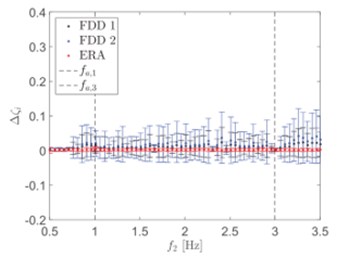
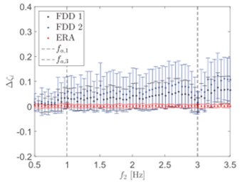
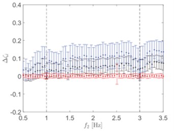
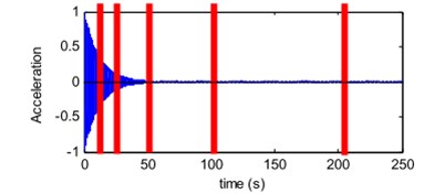
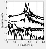
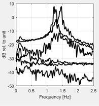
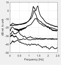
In a special case with a high level of damping, damping will be underestimated for higher modes and further amplification of underestimation occurs in the presence of signal noise as shown in Fig. 1. A high-damping system can be defined as a system with a damping ratio that is more than 1 % [20]. In actual civil structures such as a steel structure, the modal damping ratio is always higher than 1 % and the identification of modal damping is thus likely to be poorer particularly in a closely spaced mode condition. High damping ratios affect not just for closely-spaced modes but also for well-separated modes, this is caused by the peak flattening and the presence of very noisy singular values (SVs). In the previous study, generally modal damping ratios below 2 % are always used to deal with regardless of different structure characteristics [16]. However, this effect can be reduced by including additional noise modes [21]. Another problem of heavy-damped structures is that the fit becomes worse, as the nonphysical information from the noise becomes more dominant, and the correlation function decays faster. This problem can be solved by inserting extra measurement channels that can minimize the mean and standard deviation of the error and improve the identification of modal damping [21]. The new modal parameter estimation has been introduced for a high-damping system by a refined FDD algorithm, which used untended correlation functions and accounting of data filtering in the processing of a SD matrix as well as the frequency resolution effect, spectral bell width, singular value and peak selection, along with an applied-regression time window of the anti-transformed signal [16]. Besides that, Chang et al. introduced a new modal estimation method for higher damping structures by improving independent component analysis, which combined independent component analysis (ICA) with inverse damping transfer (IDT) [20].

3.3. Sensitivity to noise

A random response generated from ambient excitations on civil engineering structures is often characterized by specific variability, commonly known as the “noise,” which can lead to a bias error in modal parameter estimators. In the OMA, there is a significant issue regarding “noise” (or spurious) modes, and distinguishing them from physical modes still remains to be solved. There is also a problem associated with measurement techniques and the influences of the selection of signal processing on experimental results [22-24]. Thus, it is necessary to consider the electrical noise sources in measurement to avoid a bad signal-to-noise ratio and complexity for data analysis, which can cause a severe error in damping estimation [13]. Besides, electronic component selection, reducing noise exposure and the number of components, which are influenced by electromagnetic noise, also needs to be considered before conducting an ambient test. Certain signal processing techniques such as cyclic averaging together with root mean square (RMS) averaging can take care of random and bias errors such as leakage more effectively than regular RMS signal processing that involves overlapping and windowing [25]. The problem of a random error assessment [26] and analysis of bias error estimation [26, 27] have also been extensively discussed by the researchers recently.

Fig. 1a) Damping ratio, ζ= 0.5 %; b) damping ratio, ζ= 2 %; c) damping ratio, ζ= 5 %

a)

b)

c)

3.4. Convergence of damping estimates for higher modes

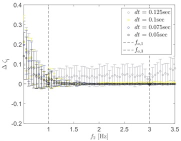
The convergence error of mean and standard deviation of damping estimation for increased frequencies of the system are the common characteristic in EFDD and mainly related to the inadequate amount of information of the decaying CF at lower frequencies of the system. It is observed that the convergence rate of the error is reliant on the time step, particularly for higher modes and it does not bring much effect to the accuracy of modal damping for the lower modes. An improved damping estimate of lower modes requires long records. For example, Fig. 2 shows the estimation errors of the second mode with variable time steps and constant time window [28]. The time step plays a crucial role to ensure the sampled data can adequately recognize the frequency component.

Fig. 2The example of mean and standard deviation of the difference between estimated a known damping for a variation of assigned natural frequencies of the systems second mode of configuration 3 using FDD. fa,1 and fa,3 are the assigned frequencies of the first and third mode. The assigned damping was 2 % and dt refers to the time step

The example of mean and standard deviation of the difference between estimated a known damping for a variation of assigned natural frequencies of the systems second mode of configuration 3 using FDD. fa,1 and fa,3 are the assigned frequencies of the first and third mode. The assigned damping was 2 % and dt refers to the time step

4. Recent development of unbiased damping ratio estimation

This section shows the recent development of EFDD procedures for unbiased modal damping estimation and a key factor to deal with.

4.1. Measurement techniques

In general, there is two essentials guideline in OMA methods: the loadings must be multiple inputs and have a good quality and length of data recorded [29].

4.1.1. Loadings

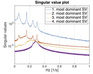
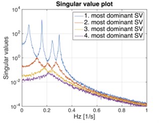
During ambient tests for a large structure, numerous sensors are applied at different locations which are already determined during simulations for capturing the essential modes of the structure. In order to produce clear multiple inputs: a loading must be moved over an entire part of the structure which is adequately able to excite all the modes and a distributed loading such as the wind with a correlation length significantly smaller than the structure [29]. There is a guideline to inspect either the structure is subjected to multiple inputs or single input which by using singular value decomposition plot. For multiple input loading, all singular value curves contribute to some extent but for single input loading, only one singular value curve is dominating, while the other singular value curves represent the noise as shown in Fig. 3 [29]. Besides, this plot can also be used to reveal the structures that have closely spaced or coincident modes.

Fig. 3Singular value decomposition plot for a 4 DOF system: a) single input loading, zero mean, Gaussian white noise applied to one DOF; b) multiple input loading, all DOFs are excited with zero mean, Gaussian white noise

Singular value decomposition plot for a 4 DOF system: a) single input loading, zero mean, Gaussian white noise applied to one DOF; b) multiple input loading, all DOFs are excited with zero mean, Gaussian white noise

a)

b)

4.1.2. Data quality and record length

The subsequent requirement that must be fulfilled is high reliable recorded data with good signal-to-noise ratio, elimination of outliers (distant observation points), dropouts, clipping and noise spikes. Spikes can be defined as noise which disturbs the measurement chain and affects the spectral density (SD) of the recorded signal by creating the higher amplitude or tails of the SD because of large peak values in the time series. On the other hand, clipping typically happens when the signal saturates the analogue digital converter and it easy to determine either by a naked eye of the time series, where the signals are cut-off at a certain amplitude, either on one or both sides or detect in the SD by large values at the end of the tails. Meanwhile, signal dropout can happen when the transmission is a loss of power, resulting in a permanent or temporarily “drop out” of the signal. This can be seen either when the amplitude of the time series signal diminishes for a period or by peaks in the SD [5].

The total length of the recorded data has played a key factor to guarantee a reliable estimate of the SD and a “rule of thumb” was presented [29]:

9

T_{t o t} = m a x (\frac{n_{d}}{ξ_{k} ω_{k}}),

where $T_{t o t}$ , $ξ_{k}$ , $ω_{k}$ and $n_{d}$ is the total record length, modal damping ratio, modal angular frequency and number of averages, respectively. The length of the record become an essential in obtaining a reliable result and has suggested at least 1 hour for ambient test on the large civil structure with first fundamental natural frequency and damping ratio of 1 Hz and 1 %, respectively [4].

In the case of fixed record length, the number of average effects the alteration of the calculated SD and corresponding singular value plot. The variation of estimated SD can be reduced for a fixed record by calculating a number of average from Eq. (9). The number of averages is significantly influence damping ratio estimation because of the half-power bandwidth and number of averages are varies proportionally to each other [29]. Besides, a high number of averages is also essential for a reliable SD estimation [29]. The high number of averages cause the convergence of damping estimate near a value which relies on the type of curve fit. The present study has revealed that if the number of average is less than 10-15 averages are adopted, damping estimates are significantly lower than this converged value [30].

4.2. Pre-processing

The important task in the signal pre-processing is to have the appropriate frequency resolution and the correct choice of the number of points of the time segments. In the following sections, we will go through the most important steps involved in this process.

4.2.1. Frequency resolution

For the estimation of modal damping, there is an indicator that can control the bias error which is called as the ratio of frequency resolution relative to the bandwidth. This can be expressed as:

10

∆ f = \frac{1}{N ∆ t}, B_{r} \approx 2 ζ f,

where $∆ f$ is the frequency resolution and $B_{r}$ is the half-power bandwidth for light damping at the resonance frequency. The high ratio $B_{r} / ∆ f$ is required to adequately estimate modal damping because less bias error is introduced by a larger ratio. The bias error may result in erroneous damping estimates, which was studied in [31].

The frequency resolution also influences the number of points used for the fit and present study recommended at least 16 points in the fit based on numerical simulations [30]. For further study regarding the effect of frequency resolution on the estimation of damping ratio via EFFD can be found in [32]. The result showed that once the frequency improves, it will affect the true estimation of damping ratio for all identified modes. In order to decrease the frequency resolution, the total length of the acquisitions should be extended, despite it would increase the number of computations. In particular, convergence is found for a frequency resolution equal to 0.01 Hz or better. In the present study, they stated that the appropriate results can be achieved if time recordings lasting about 1000-2000 times the first natural period of the structure [29].

4.2.2. Number of points of the time segments

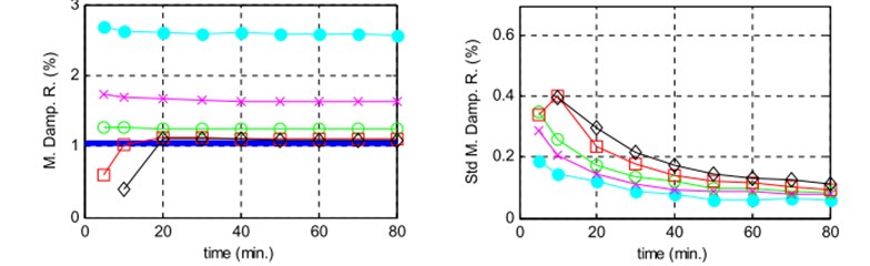
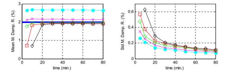
The correct choice of the number of points of the time segments is essential because it has a stronger influence on the results, otherwise, it can lead to high bias errors (more than 100 %). This is related to the sufficient amount of information of the decaying CF for estimating modal damping. If the estimated CF does not contain some points after the vanishing of the decay, this shows that the length of the estimated CF is not adequate enough to characterize the full decay and brought to errors in the estimation of the spectra which can affect the modal damping results [33]. This case was studied by Filipe Magalhães with varying the total duration of the acceleration time series from 5 to 80 minutes and using five alternative time segments lengths that have been defined in Table 1 and with the scheme presented in Fig. 5 clearly proves the claim related to the limits of the auto-CF calculated using different time segment lengths [4, 34]. The bias can clearly see before the end of the decay for the 128 and 256 number of the points of the time segments of the first mode (-●- and -x- lines of the top left the plot of Fig. 4).

Table 1Scenarios for the application of the EFDD method

Number of points of the time segments	Total time length (minutes)
Number of points of the time segments	5	10	20	30	40	50	60	70	80
128 (-●-)*	1a	1b	1c	1d	1e	1f	1g	1h	1i
256 (-x-)*	2a	2b	2c	2d	2e	2f	2g	2h	2i
512 (-○-)*	3a	3b	3c	3d	3e	3f	3g	3h	3i
1024 (-□-)*	4a	4b	4c	4d	4e	4f	4g	4h	4i
2048 (-◊-)*	–	5b	5c	5d	5e	5f	5g	5h	5i
* symbols used in the graphics of Fig. 4

Fig. 4Mean values and standard deviations of the estimates obtained with the standard algorithm of the EFDD method for the 2 modes using the parameters characterized in Table 1. a) Mode 1, b) mode 2 theoretical values represented by a horizontal solid line, symbol of the lines defined in Table 1

Mean values and standard deviations of the estimates obtained with the standard algorithm of the EFDD method for the 2 modes using the parameters characterized in Table 1. a) Mode 1, b) mode 2 theoretical values represented by a horizontal solid line, symbol of the lines defined in Table 1

a)

b)

Fig. 5The theoretical modal decay of the first mode and limits of the auto-correlation functions calculated using the time segment lengths defined in Table 1

The theoretical modal decay of the first mode and limits of the auto-correlation functions calculated using the time segment lengths defined in Table 1

Hence, the correct choice of the time segments length reliant on the natural frequencies and modal damping ratios of the modes under analysis. Lower natural frequencies and lower modal damping ratios require longer time segments. The plots of Fig. 4. indicate that the total time length should be longer than 20 minutes in order to demand reliable damping estimate. By increasing the total time length, the number of averaging can be increased and indirectly cause the standard deviation to reduce.

4.3. Signal processing

Generally, signal processing is used to provide a clearer picture of the physical problem that we are dealing with. With a proper selection of signal processing techniques, all essential information about the system, that is, the modal parameters for each mode (the mode shape, the natural frequency, and the modal damping ratio) can be extracted from the raw signal through estimation of correlation functions (CF) and spectral densities (SD).

4.3.1. Correlation function estimation

There are two basic assumptions associated with CF. First, all (or nearly all) the information about the modal characteristics from the random signal are extracted by CF and besides that, this CF can be expressed as free decays of the system. Hence, estimation of CF is fundamental in OMA.

The easiest way of estimating unbiased CF is via direct estimation and it became more desirable due to its ability to perform the unbiased estimation by simple means. However, it has a drawback in term of calculation time consuming compared with other estimation techniques.

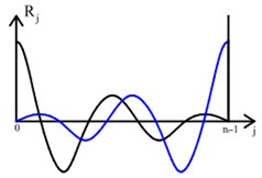
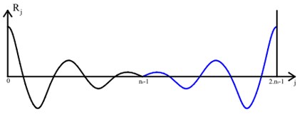
Besides, one of the most well-known ways of estimating CF is using the Welch method. Data segmenting and subsequent Fourier transform of each data segment are used in this method and all these individual data segments are assumed to be periodic. The assumption of periodicity able to reduce discontinuities at the ends, otherwise it will lead to the leakage bias, where frequencies carrying high energy. This bias can also be denoted as a “leakage error”. See Brandt [17] for a detailed description of the leakage error and how to minimize it. Moreover, this method also may cause noisier SVs as well as produce circular correlations which become a superposition of the desired function and its mirror image of calculated correlation as shown in Fig. 6(a) due to the process of signal sectioning, windowing and overlapping [35-37]. This circular error can significantly lead to the bias estimates of modal parameters, particularly modal damping ratio.

The following approach is using unbiased Welch estimate. This approach is implemented to overcome the problem of circular error in Welch method by doubling the length of the time segments and add zeros at the end (this process produces a translation of the mirrored correlation from the position at the left to the position at the right side in Fig. 6) [35, 38]. Before that, time segments from the measured signals without the use of windows need to be well chosen.

Fig. 6a) Circular correlation, b) correlation calculated by doubling the length of the time segments and add zeros at the end

a)

b)

The fast and simple of random decrement (RD) method for estimation of CF by simple mean of time averaging is also popular among researchers in the case of system parameter identification [39]. The basic idea of the method is to estimate a so-called RD signature which estimated by averaging segments from the signal, where the signal at the time steps satisfy the triggering condition and the number of triggering points. The process of this algorithm is illustrated in Fig. 7. From this fundamental solution, it is possible to explain the meaning of the RD signature for several triggering conditions of practical interest, see Table 2. The different use of RD triggering conditions to capture the data segments around the triggering points and averaging them to form the signature able to estimate modal parameters with different amplitude levels. Further information about the RD technique together with information about uncertainty estimating of the RD signature can be obtained in [40].

Fig. 7Estimation of a random decrement signature by defining a triggering condition

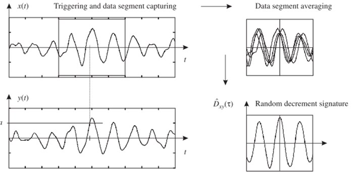
Table 2Commonly used RD triggering conditions and their effects condition

Condition name	Triggering condition	Effect on RD estimates
Level crossing	$y (t) = a$	$D_{x y} (τ) \propto R_{y x} (τ)$
Level band	$y (t) \in [a_{1}; a_{2}]$	$D_{x y} (τ) \propto R_{y x} (τ)$
Velocity crossing	$\dot{y} (t) = v$	$D_{x y} (τ) \propto {\dot{R}}_{y x} (τ)$
Positive points	$y (t) > a$	$D_{x y} (τ) \propto R_{y x} (τ)$
Positive velocity	$\dot{y} (t) > v$	$D_{x y} (τ) \propto {\dot{R}}_{y x} (τ)$

4.3.2. Tapering (windowing)

The FFT algorithm requires windows to reduce leakage in SD by forcing the endpoints of each signal sample data to zero. The use of windows will on average reduce the bias but cannot completely remove it due to the change in the half-power bandwidth [34]. There are different options for the choice of the time windows functions in literature, but in this review only discusses or highlight the commonly used time windows functions in OMA.

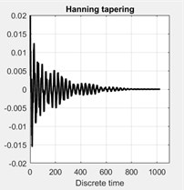
The Hanning window with 50 % overlap is the most common ones used in signal processing and capable to reduce leakage effects in spectrum computation, instead, this is not an optimal solution and produces a bias error with respect to the true damping value. It is nevertheless a reasonable choice in all OMA cases. The bias error in the estimation of the SD using a Hanning window was studied in detail in [8, 41].

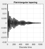
Besides that, the use of flat-triangular window can moderately reduce the side lobe noise. In this case, a value of $α =$ 0.5 was used in this application of moderate tapering. As tapered by an exponential window that is reduced to 0.05 % at the boundaries.

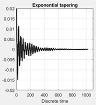
Moreover, the application of a classical exponential window able to significantly reduce the side lobe noise with 5 % of the initial value at the boundaries, however, it will lead to the appearance of a clear bias at the spectral peaks.

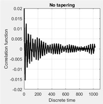
The resulting tapered correlation functions and corresponding spectral density with a different application of tapering (windowing) are shown in Fig. 8. This figure shows that the application of time window able to illustrates the spectral peaks more clearly, instead, yields a clear bias of the spectral peaks.

Fig. 8Effect of application of different tapering (windowing). Top plots show the autocorrelation function for the four cases of tapering: a) without any tapering, b) tapered by Hanning window, c) with the flat-triangular window, d) by an exponential window. e)-f) show the corresponding spectral density plots of the singular values of the spectral matrix

Effect of application of different tapering (windowing). Top plots show the autocorrelation function for the four cases of tapering: a) without any tapering, b) tapered by Hanning window, c) with the flat-triangular window, d) by an exponential window. e)-f) show the corresponding spectral density plots of the singular values of the spectral matrix

a)

b)

c)

d)

e)

f)

g)

h)

4.3.3. Spectral density estimation

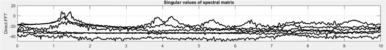
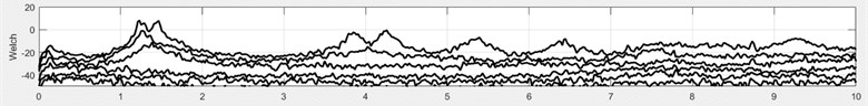
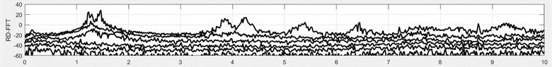
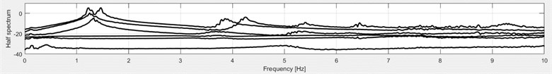
Estimation of damping ratios is highly reliant on the singular value plot, attained by singular value decomposition (SVD) from the estimated SD. The errors and variability in the estimated SD which typically come from windowing and frequency resolution will highly affect the estimation of damping ratios [5]. Fig. 9 depict the singular values of the SD matrix with different ways of approach.

The top plot of Fig. 9 shows the SD obtained from the direct estimates of the correlation function matrix, multiplied by the flat-triangular window with $α =$ 0.5 and then transformed by the FFT. The second plot from the top is the traditional Welch averaging with a Hanning window and 50 % overlap, obtained by signal sectioning, windowing and overlapping. The third plot from the top is the RD estimate obtained by using band triggering with a symmetric band around zero and a width of ±2 $σ$ ,where $σ$ is the standard deviation of the triggering signal and it does not need any windowing because the natural decay of the RD functions removes the need for windowing. It should be noted that the scale of the RD spectral estimate is different due to the fact that the initial value of the RD function depends on the triggering condition. The bottom plot is the half spectrum derived based in the zero-padded direct correlation function estimate, multiplied by the flat-triangular window and then transformed by the FFT. It can produce smoother and clearer result of the desired physical information than any of the other estimates. Basically, all four ways of estimating the SD give us the same information of spectral representations of the modes, however, if too much suppress the side lobe noise such as in the half spectrum, it will affect the true modal damping values and appearance of a clear bias at the spectral peaks because each modal peak is corresponding to the damping.

4.4. Identified single degree of freedom (SDOF) bell functions

There are two ways to identify SDOF bell function before transferring back to the time domain by using inverse Fourier Transform.

First is by setting boundary condition for the selected peak of singular values. However, this require experienced technical person to properly set the boundary for a selected peak in order to extract all the useful information. Generally, the width of the frequency band to be used for identification is 1 Hz [42]. The second approach is by using modal assurance criterion analysis (MAC) technique which quantifies the comparison of two mode shapes. The MAC value of one or 100 % indicates that the mode shapes are identical (equivalent movement of all points) meanwhile the MAC value that closes to zero will have dissimilar mode shapes. The previous algorithm typically used MAC value lesser than 0.90 which can cause deviation of the natural frequency estimates almost 5 % and also affect the estimation of damping ratio for the heavy-damped cases up to 30 % deviation for the first modes, while frequently fail for the higher modes. Therefore, the appropriate MAC values with remarkable mode shape estimates should be greater than 0.95 [16].

Fig. 9Singular values of the spectral density matrix with different signal processing approach. All plots are in dB relative to the measurement unit. a) The Fourier transformed direct estimate of the correlation functions; b) the traditional Welch averaging with a Hanning window and 50 % overlap; c) the RD estimate; d) the half spectrum based on the zero-padded direct correlation function matrix estimate

Singular values of the spectral density matrix with different signal processing approach. All plots are in dB relative to the measurement unit. a) The Fourier transformed direct estimate of the correlation functions; b) the traditional Welch averaging with a Hanning window and 50 % overlap; c) the RD estimate; d) the half spectrum based on the zero-padded direct correlation function matrix estimate

a)

b)

c)

d)

4.5. Time window selection and extrema picking

The selection of the accurate time window on the SDOF Auto-Correlation Function (ACF) is a bit challenging and the hard part of the algorithm. Together with the spectral bell identification, only one separated segment involves in these process through inverse FFT and bias errors might likely occur in damping estimates. This drawback must be considered particularly for closely spaced modes [43]. In order to attain a clear time window representation, contents, decimation and frequency resolution must be well chosen. Besides, the reliable result of the linear regression operation with respect to the adequacy of the time window selection.

The classical way for time window selection is by putting the number of points to be used for identification of damping on the modal coordinate in the time domain. All extrema, i.e. peaks and valleys, act as the free decay of a damped SDOF system, are determined within a suitable time window (for example 90 % to 20 % of the maximum amplitude). In a recent study, the iterative operation of advanced optimization which computationally efficient procedure with an integrated double loop, has been proposed to correctly choose the spectral bell identification and the clear time window representations in autonomous ways. This procedure showed is capability of reducing errors and yield accurate estimates of the modal damping ratios, particularly for the major issues of non-stationary input and high damping compared with classical EFDD procedures [4, 33, 44].

4.6. Techniques for modal damping estimation

There are a variety of methods for measuring the damping of a vibration system. The simple way and fast to estimate damping ratio from frequency domain are by using half-power bandwidth method. Half-power bandwidth is defined as the ratio of the frequency range between the two half-power points to the natural frequency at this mode. However, it has Low accuracy in computation of damping ratio due to a biased result and inapplicability to a closely spaced mode system. The classical logarithmic decrement (LogDec) method is commonly used to give a quick estimate of the modal damping ratio and provide more accurate results compared with half-power bandwidth method. LogDec is the natural logarithmic value of the ratio of two adjacent peak values of displacement in free decay vibration. Possible appearance of beat phenomena, which cause poor computation of the damping ratio, in the case of closely spaced modes and polluted with noise. Besides, the use of Hilbert transform (HT) for estimating modal damping is more efficient than the previous approach because it only requires one data block with sufficient points to obtain a good estimate of damping ratio, even noise is presented [13]. Moreover, natural excitation techniques (NExt) such as cross-covariance function, Ibrahim time domain, and Polyreference are also popular among researchers for modal damping estimation [45]. The cross-covariance function can provide a better result with a less time-consuming and unbiased estimation, even in the case of closely spaced modes. Meanwhile, Ibrahim time domain and Polyreference are simple but influenced by the closely coupled modes and noisy signal. An approach based on modified morlet wavelet capable to minimize leakage and random error but the possibility to estimate accurate modal damping due to an erroneous selection of the optimal wavelet [46].

Table 3Summarized of existing approaches for each step in enhanced frequency domain decomposition (EFDD)

Aspects			Advantages	Disadvantages
Time window	Hanning		It is nevertheless a reasonable choice in all OMA cases and the most commonly employed window	Implies a loss factor of 3/8 and increases the half power bandwidth of the main lobe, thus can produce a bias error with respect to the true damping value
	Triangular		Capable to reduce bias error in modal damping estimate	The side lobe noise is moderately reduced
	Exponential		The side lobe noise is significantly reduced with 5 % of the initial value at the boundaries	Lead to the appearance of a clear bias at the spectral peaks
Correlation function and spectral density estimate	Direct estimation		The easiest way of estimating unbiased CF and it became more desirable to use	It has a drawback in term of calculation time consuming compared with other estimation techniques
	Welch method		Less computational demanding	The leakage bias is introduced by the wrong assumption of periodicity. The implementation of signal sectioning, windowing and overlapping but sometimes may lead to noisier SVs. It requires some operations on the signal in order to improve the quality of the estimates
	Unbiased Welch estimate		Implement the Welch method using zero padding in such a way that the leakage error on the correlation functions vanishes completely	The leakage bias is introduced by the wrong assumption of periodicity. It requires some operations on the signal in order to improve the quality of the estimates
	Random decrement (RD) technique		The noise reduction by averaging the time segments of the raw signals and it does not need any windowing because the natural decay of the RD functions	Produce high side lobe noise and the scale of the RD spectral estimate is different due to the fact that the initial value of the RD function depends on the triggering condition
	Half spectra		The half spectrum is smoother and thus gives a clearer picture of the desired physical information of estimating the SD than any of the other estimates	Yields a clear bias at the spectral peaks
Identified SDOF Bell Functions	Set boundary for selected peak		Capable to select and identify SDOF bell functions efficiently	Need to properly set the boundary for selected peak and require experienced technical person in order to extract all the information
	Modal assurance criterion analysis (MAC)		One of the most popular tools for the quantitative comparison of modal vectors and able to use of autonomous estimation of modal parameters. The appropriate MAC values with remarkable mode shape estimates should be greater than 0.95	Even though, the appropriate MAC values with remarkable mode shape estimates should be greater than 0.95, but need to properly set the MAC values from the range 0.95 until 1
Time window selection and extrema picking	Set suitable time window and boundary		Easy to implement by setting the constant number of points to be used for identification of damping on the each modal coordinate in the time domain. A suitable time window (for example 90 % to 20 % of the maximum amplitude) were taken	Need to properly set the suitable time window and extrema picking. Require expertised or technical person
	Iterative loop & advanced optimization algorithm		The selection of the correct time window on the SDOF auto-correlation Function (ACF) and the choice of the spectral bell can be performed	High computational demanding and time consuming
Techniques for modal damping estimation	Half Power Bandwidth Method		No interfere with the calculation modes; faster and easier use	Lower accuracy in computation of damping ratio due to a biased result; inapplicability to a closely spaced mode system
	Logarithmic Decrement		A commonly used method, user-friendly and fast processing algorithm	Possible appearance of beat phenomena, which cause poor computation of the damping ratio, in the case of closely spaced modes and polluted with noise. It can deal only with SDOF system
	Hilbert Transform (HT)		Only one data block with sufficient points is required to obtain a good estimate of damping ratio, even noise is presented	It can deal only with SDOF system
	Natural Excitation Technique	Cross-covariance function	Allow a better result with a less time-consuming with higher computational speed and unbiased estimation, even in the case of closely spaced modes	The approach is not numerically robust and produce high uncertainties due to matrix squared up
		Ibrahim TD	Powerful estimation of modal damping for simulation and simpler to use	Influenced by the closely coupled modes and noisy signal
		Polyreference	Clear and fast stabilisation diagrams that are easier to interpret	Poor estimation of modal damping when noise level increases and influenced by closely spaced mode
	Modified Morlet Wavelet		High accuracy of the estimation of modal damping from weak or strong vibration responses as well as long and short duration records and also has capability to minimize leakage and random error	Possibility to estimate accurate modal damping due to an erroneous selection of the optimal wavelet

5. Conclusions

The user-friendly and fast processing algorithm of enhanced frequency domain decomposition (EFDD) indicates that it capable of providing reliable results but with the condition of good selection of parameters for spectra computation and well-separated modes [4]. However, this method has drawbacks in providing an accurate estimation of damping ratios, despite natural frequencies and mode shapes can be computed through assuredly and reasonably accurate estimates [3]. The exact practical computation of modal damping is still an open issue, often leading to biased estimates since the errors are coming from every step in EFDD procedures and mainly due to signal processing [5]. The rapid development of EFDD method justifies the need for more comprehensive review studies, in order to find the best practice criteria for modal parameter identification and provide relevant essential information on modal damping for a reliable estimation, reduce uncertainties and define error bounds. First, steps of classical enhanced FDD algorithm for modal parameter estimation was addressed. An extensive literature has been used in the current study to help researchers get introduced to the subject of OMA particularly EFDD method and provide essential information regarding the factors that contribute to unbiased estimate and the ways to overcome this issue. Further research can be conducted to improve the estimation modal damping in OMA using valuable and essential information provided by the current study.

References

Zhang L., Brincker R., Andersen P. An overview of operational modal analysis: major development and issues. Proceedings of the 1st International Operational Modal Analysis Conference, Copenhagen, Denmark, 2005, p. 179-190.

Search CrossRef
Mironov A., Doronkin P., Priklonsky A., Kabashkin I. Condition monitoring of operating pipelines with operational modal analysis application. Transport and Telecommunication Journal, Vol. 16, Issue 4, 2015, p. 305-319.

Publisher
Rainieri C., Fabbrocino G. Learning operational modal analysis in four steps. Proceeding of the 6th International Operational Modal Analysis Conference, Gijón, Spain, 2015.

Search CrossRef
Magalhães F., Cunha Á., Caetano E., Brincker R. Damping estimation using free decays and ambient vibration tests. Mechanical Systems and Signal Processing, Vol. 24, Issue 5, 2010, p. 1274-1290.

Publisher
Rainieri C., Fabbrocino G. Operational Modal Analysis of Civil Engineering Structures. Springer, New York, 2014.

Publisher
Rainieri C., Fabbrocino G., Cosenza E. On damping experimental estimation. Proceedings of the 10th International Conference on Computational Structures Technology, 2010.

Search CrossRef
Chen B., Zhang Z., Hua X., Basu B., Nielsen S. R. K. Identification of aerodynamic damping in wind turbines using time-frequency analysis. Mechanical Systems and Signal Processing, Vol. 91, Issue 5, 2017, p. 198-214.

Publisher
Bendat J. S., Piersol A. G. Random Data: Analysis and Measurement Procedures. John Wiley and Sons, Hoboken, 2011.

Publisher
Maia N. M. M., Silva J. M. M. Theoretical and Experimental Modal Analysis. Research Studies Press, Tounton, England, 1997.

Search CrossRef
Pioldi F. On the Formulation of Optimized Algorithms of Modal Dynamic Identification and Their Application in Seismic Field. M.Sc. Thesis, University of Bergamo, 2013.

Search CrossRef
Brincker R., Zhang L. Frequency domain decomposition revisited. Proceedings of the 3rd International Operational Modal Analysis Conference, Portonovo, Italy, 2009, p. 615-626.

Search CrossRef
Gade S., Møller N. B., Herlufsen H., Konstantin Hansen H. Frequency domain techniques for operational modal analysis. Proceedings of the 1st International Operational Modal Analysis Conference, Copenhagen, Denmark, 2005, p. 261-271.

Search CrossRef
Zhang L., Tamura Y. Damping estimation of engineering structures with ambient response measurements. Proceedings of the 21st International Modal Analysis Conference, Kissimmee, Florida, 2003.

Search CrossRef
Jacobsen N., Andersen P., Bricker R. Applications of frequency domain curve-fitting in the EFDD technique. Proceedings of the 26th International Modal Analysis Conference, Orlando, Florida, 2008.

Search CrossRef
Rodrigues J., Brincker R., Andersen P. Improvement of frequency domain output-only modal identification from the application of the random decrement technique. Proceedings of the 23rd International Modal Analysis Conference, Dearborn, Michigan, 2004.

Search CrossRef
Pioldi F., Ferrari R., Rizzi E. Output-only modal dynamic identification of frames by a refined FDD algorithm at seismic input and high damping. Mechanical Systems and Signal Processing, Vol. 68, Issue 69, 2016, p. 265-291.

Publisher
Brandt A. Noise and Vibration Analysis: Signal Analysis and Experimental Procedures. John Wiley and Sons, Chichester, 2011.

Publisher
Jeary A. P. Damping in tall buildings – a mechanism and a predictor. Earthquake Engineering and Structural Dynamics, Vol. 14, Issue 5, 1986, p. 733-750.

Publisher
Tamura Y., Zhang L., Yoshida A., Nakata S., Itoh T. Ambient vibration tests and modal identification of structures by FDD and 2DOF-RD technique. Structural Engineers World Congress, Yokohama, Japan, 2002.

Search CrossRef
Chang J., Liu W., Hu H., Nagarajaiah S. Improved independent component analysis based modal identification of higher damping structures. Measurement, Vol. 88, 2016, p. 402-416.

Publisher
Bajric A., Georgakis C. T., Brincker R. Evaluation of damping using time domain OMA techniques. Proceedings of 2014 SEM Fall Conference and International Symposium on Intensive Loading and Its Effects, Beijing, China, 2014.

Search CrossRef
Farrar C. R., Doebling S. W., Cornwell P. J. A comparison study of modal parameter confidence intervals computed using the Monte Carlo and Bootstrap techniques. Proceeding of SPIE – The International Society for Optical Engineering, Vol. 2, 1998, p. 936-944.

Search CrossRef
Lamb M., Rouillard V. Some issues when using Fourier analysis for the extraction of modal parameters. Journal of Physics: Conference Series, Vol. 181, 2009, p. 012007.

Search CrossRef
Özşahin O., Özgüven H. N., Erhan B. Analysis and compensation of mass loading effect of accelerometers on tool point FRF measurements for chatter stability predictions. International Journal of Machine Tools and Manufacture, Vol. 50, Issue 6, 2010, p. 585-589.

Publisher
Chauhan S., Phillips A. W., Allemang R. J. Damping estimation using operational modal analysis. Proceedings of the 26th International Modal Analysis Conference, Orlando, Florida, 2008.

Search CrossRef
Giampellegrini L., Greening P. Estimation errors in operational modal analysis. Proceedings of the 1st International Operational Modal Analysis Conference, Copenhagen, Denmark, 2005.

Search CrossRef
Berczyński S., Chmielewski K., Chodźko M. Analysis of bias of modal parameter estimators. Advances in Manufacturing Science and Technology, Vol. 36, Issue 3, 2012, p. 19-27.

Search CrossRef
Bajric A., Brincker R., Thöns S. Evaluation of damping estimates in the presence of closely spaced modes using operational modal analysis techniques. Proceedings of the 6th International Operational Modal Analysis Conference, Gijon, Spain, 2015.

Search CrossRef
Brincker R., Ventura C., Andersen P. Why output-only modal testing is a desirable tool for a wide range of practical applications. Proceedings of the 21st International Modal Analysis Conference, The Hyatt Orlando, Kissimmee, Florida, p. 265-2003.

Search CrossRef
Brownjohn J. M. W. Assessment of Structural Integrity by Dynamic Measurements. Ph.D. Thesis, University of Bristol, 1988.

Search CrossRef
Brownjohn J. M. W. Estimation of damping in suspension bridges. Proceedings of the ICE – Structures and Buildings, Vol. 104, Issue 4, 1994, p. 401-415.

Publisher
Tamura Y., Yoshida A., Zhang L., Ito T., Nakata S., Sato K. Examples of modal identification of structures in Japan by FDD and MRD techniques. Proceedings of the 1st International Operational Modal Analysis Conference, Copenhagen, Denmark, 2005.

Search CrossRef
Brincker R., Ventura C. E., Andersen P. Damping estimation by frequency domain decomposition. Proceedings of the 19th International Modal Analysis Conference, Hyatt Orlando, Kissimmee, Florida, Vol. 1, 2001, p. 698-703.

Search CrossRef
Magalhães F. Operational Modal Analysis for Testing and Monitoring of Bridges and Special Structures. Ph.D. Thesis, University of Porto, 2010.

Search CrossRef
Bendat J. S., Piersol A. G. Engineering Applications of Correlation and Spectral Analysis. Wiley-Interscience, New York, 1980.

Search CrossRef
Welch P. D. The use of Fast Fourier Transform for the estimation of power spectra: a method based on time averaging over short, modified periodograms. IEEE Transactions on Audio and Electroacoustics, Vol. 15, Issue 2, 1967, p. 70-73.

Publisher
Pioldi F., Ferrari R., Rizzi E. A refined FDD algorithm for operational modal analysis of buildings under earthquake loading. Proceedings of the 26th International Conference on Noise and Vibration Engineering, Leuven, Belgium, Vol. 1, 2014, p. 3353-3368.

Search CrossRef
Brincker R., Krenk S., Kirkegaard P. H., Rytter A. Identification of Dynamical Properties from Correlation Function Estimates. Danish Society for Structural Science and Engineering, Aalborg, 1992.

Search CrossRef
Rodriguez J., Brincker R. Application of the random decrement technique in operational modal analysis. Proceedings of the 1st International Operational Modal Analysis Conference, Copenhagen, Denmark, 2005, p. 191-200.

Search CrossRef
Asmussen J. C. Modal Analysis Based on the Random Decrement Technique – Application to Civil Engineering Structures. Ph.D. Thesis, University of Aalborg, 1997.

Search CrossRef
Schmidt H. Resolution bias errors in spectral density, frequency response and coherence function measurements, I: General theory. Journal of Sound and Vibration, Vol. 101, Issue 3, 1985, p. 347-362.

Publisher
Bricker R., Venture C. Introduction to Operational Modal Analysis. John Wiley and Sons, Chichester, 2015.

Publisher
Zhang L., Wang T., Tamura Y. A frequency-spatial domain decomposition (FSDD) method for operational modal analysis. Mechanical Systems and Signal Processing, Vol. 24, Issue 5, 2010, p. 1227-1239.

Publisher
Brincker R., Zhang L., Andersen P. Output-only modal analysis by frequency domain decomposition. Proceedings of the 25th International Seminar on Modal Analysis, Leuven, Belgium, Vol. 2, 2000, p. 717-724.

Search CrossRef
Anela B., Georgakis T. C., Brincker R. Evaluation of damping using frequency domain operational modal analysis techniques. Proceedings of the 33rd International Modal Analysis Conference, Orlando, Florida, Vol. 2, 2015, p. 351-355.

Search CrossRef
Tarinejad R., Damadipour M. Modal identification of structures by a novel approach based on FDD-wavelet method. Journal of Sound and Vibration, Vol. 333, Issue 3, 2014, p. 1024-1045.

Publisher

Cited by

LSTM-Based Approach for Stable Identification of Modal Damping Ratio in Building Structures

Da Yo Yun | Byung Kwan Oh | Kanghyun Park | Hyo Seon Park | Yongchao Yang

(2024)

Research Progress on Dynamic Characteristic Monitoring Methods of Super High-Rise Buildings

Yongjingbang WU | Nan JIN | Zhongqi SHI | Qingrui YUE | Rumian ZHONG

(2024)

Output-Only Modal Identification Based on Auto-regressive Spectrum-Guided Symplectic Geometry Mode Decomposition

Pengming Zhan | Xianrong Qin | Qing Zhang | Yuantao Sun

(2024)

Recent vibration-based structural health monitoring on steel bridges: Systematic literature review

Anis Shafiqah Azhar | Sakhiah Abdul Kudus | Adiza Jamadin | Nur Kamaliah Mustaffa | Kunitomo Sugiura

(2024)

Identification of temperature-dependent elastic and damping parameters of carbon–epoxy composite plates based on experimental modal data

(2023)

Two-step online identification of in-service cable-inertial mass damper systems under nonstationary wind excitations

Xiongjun Yang | Ying Lei | Lijun Liu | Hongping Zhu | Wenai Shen

(2023)

Structural Damping Ratio Identification through Iterative Frequency Domain Decomposition

Chun-Xu Qu | Yu-Fei Liu | Ting-Hua Yi | Hong-Nan Li

(2023)

SSI-LSTM network for adaptive operational modal analysis of building structures

Da Yo Yun | Hak Bo Shim | Hyo Seon Park

(2023)

Modal and Structural Identification of Historic Bell Tower in Čuntić, Croatia Using Ambient Vibration Testing

Marina Sunara | Ivan Banović | Ante Buzov | Nikola Grgić

(2023)

Vibration-Based and Near Real-Time Seismic Damage Assessment Adaptive to Building Knowledge Level

(2022)

Experimental Investigation on Dynamic Characteristics Changes of Fire Exposed Reinforced Concrete and Steel Members

(2022)

Structural health monitoring and modal parameters identification of Mezcala Bridge

Anaya-Diaz Miguel | Carrion-Viramontes Francisco J | Quintana-Rodriguez Juan A | Martinez-Trujano Luis A | Machorro-Lopez Jose M

(2022)

Ambient vibration testing and seismic fragility analysis of masonry building aggregates

(2022)

Automated operational modal analysis based on long‐term records: A case study of Milad Tower structural health monitoring

Amirali Sadeqi | Akbar Esfandiari | Masoud Sanayei | Mohammad Rashvand

(2022)

Application of operational modal analysis to investigate transformer vibration patterns

Jakob Pallot | Chandima Ekanayake | Hui Ma | Lakshitha Naranpanawe

(2022)

Development of a low cost system for modal parameters identification under ambient vibration: A low rise building as a case study

Mina Derife | Abderrahman Atmani | El Hassan Ait Laasri | Jama Balil | Driss Agliz

(2022)

Design, fabrication, and dynamic testing of a large-scale outdoor aeroelastic model of a long-span cable-stayed bridge

Zhaoyu Ma | Fuyou Xu | Miaomin Wang | Mingjie Zhang | Hua Zeng

(2022)

Field measurements for identification of modal parameters for high-rise buildings under construction or in use

(2021)

Assessment of modal characteristics of cross-laminated timber beams subject to successive damages

Ali Fuat Genç | Volkan Kahya | Ahmet Can Altunışık | Murat Günaydın | Cenk Demirkır

(2021)

A review of operational modal analysis techniques for in-service modal identification

Fahad Bin Zahid | Zhi Chao Ong | Shin Yee Khoo

(2020)

Field test investigations for condition monitoring of a concrete culvert bridge using vibration responses

Solomon T.K. Lin | Ye Lu | Mehrisadat Makki Alamdari | Nguyen L.D. Khoa

(2020)

About this article

Received

06 September 2017

Accepted

05 February 2018

Published

15 August 2018

SUBJECTS

Mechanical vibrations and applications

DOI

https://doi.org/10.21595/jve.2018.19058

Keywords

operational modal analysis

damping estimation

Acknowledgements

The authors would like to extend their greatest gratitude to the Institute of Noise and Vibration UTM for funding the current study under the Higher Institution Centre of Excellence (HICoE) Grant Scheme (R.K130000.7843.4J227). Additional funding for this research came from the UTM Research University Grant (Q.K130000.2543.11H36) and the Fundamental Research Grant Scheme (R.K130000.7840.4F653) from The Ministry of Higher Education, Malaysia.

This is an open access article distributed under the Creative Commons Attribution License, which permits unrestricted use, distribution, and reproduction in any medium, provided the original work is properly cited.

Next article in issue Next

Research article

2023 09 21

Automatic modal identification of bridges based on free vibrations and advanced signal decomposition techniques

Matteo Mazzeo, Dario De Domenico, Giuseppe Quaranta, Roberta Santoro

Research article

2020 12 04

Damping estimation of a pedestrian footbridge – an enhanced frequency-domain automated approach

Basuraj Bhowmik, Budhaditya Hazra, Michael O’Byrne, Bidisha Ghosh, Vikram Pakrashi

Research article

2020 05 07

Methods to enhance the automation of operational modal analysis

Marcel Wiemann, Lukas Bonekemper, Peter Kraemer

Research article

2020 03 23

Identification of non-proportional structural damping using experimental modal analysis data

Akın Oktav

M. D. A. Hasan, Z. A. B. Ahmad, M. Salman Leong, and L. M. Hee, “Enhanced frequency domain decomposition algorithm: a review of a recent development for unbiased damping ratio estimates,” Journal of Vibroengineering, Vol. 20, No. 5, pp. 1919–1936, Aug. 2018, https://doi.org/10.21595/jve.2018.19058

Copy Extrica

Copied to clipboard!

TY  - JOUR
DO  - 10.21595/jve.2018.19058
UR  - https://doi.org/10.21595/jve.2018.19058
TI  - Enhanced frequency domain decomposition algorithm: a review of a recent development for unbiased damping ratio estimates
T2  - Journal of Vibroengineering
AU  - A. Hasan, M. Danial
AU  - Ahmad, Z. A. B.
AU  - Salman Leong, M.
AU  - Hee, L. M.
PY  - 2018
DA  - 2018/08/15
PB  - JVE International Ltd.
SP  - 1919-1936
IS  - 5
VL  - 20
SN  - 1392-8716
SN  - 2538-8460
ER  - 

Copy Ris

Copied to clipboard!

@article{A_Hasan_2018,
	doi = {10.21595/jve.2018.19058},
	url = {https://doi.org/10.21595/jve.2018.19058},
	year = 2018,
	month = {aug},
	publisher = {{JVE} International Ltd.},
	volume = {20},
	number = {5},
	pages = {1919--1936},
	author = {M. Danial A. Hasan and Z. A. B. Ahmad and M. Salman Leong and L. M. Hee},
	title = {Enhanced frequency domain decomposition algorithm: a review of a recent development for unbiased damping ratio estimates},
	journal = {Journal of Vibroengineering}
}

Copy Bibtex

Copied to clipboard!

[1]M. D. A. Hasan, Z. A. B. Ahmad, M. Salman Leong, and L. M. Hee, “Enhanced frequency domain decomposition algorithm: a review of a recent development for unbiased damping ratio estimates,” Journal of Vibroengineering, vol. 20, no. 5, pp. 1919–1936, Aug. 2018, doi: 10.21595/jve.2018.19058.

Copy IEEE

Copied to clipboard!

A. Hasan, M. Danial, Z. A. B. Ahmad, M. Salman Leong, and L. M. Hee. “Enhanced Frequency Domain Decomposition Algorithm: A Review of a Recent Development for Unbiased Damping Ratio Estimates.” Journal of Vibroengineering 20, no. 5 (August 15, 2018): 1919–36. https://doi.org/10.21595/jve.2018.19058.

Copy Chicago

Copied to clipboard!

Enhanced frequency domain decomposition algorithm: a review of a recent development for unbiased damping ratio estimates

Abstract

1. Introduction

2. Theoretical framework of EFDD techniques

3. Evaluation of modal damping estimation using EFDD

3.1. Damping estimation error

3.2. High level of damping

3.3. Sensitivity to noise

3.4. Convergence of damping estimates for higher modes

4. Recent development of unbiased damping ratio estimation

4.1. Measurement techniques

4.1.1. Loadings

4.1.2. Data quality and record length

4.2. Pre-processing

4.2.1. Frequency resolution

4.2.2. Number of points of the time segments

4.3. Signal processing

4.3.1. Correlation function estimation

4.3.2. Tapering (windowing)

4.3.3. Spectral density estimation

4.4. Identified single degree of freedom (SDOF) bell functions

4.5. Time window selection and extrema picking

4.6. Techniques for modal damping estimation

5. Conclusions

References

Cited by

About this article

Related Articles