Methods to enhance the automation of operational modal analysis

1. Introduction

The Stochastic Subspace Identification (SSI) Algorithm is widely used in modal analysis to identify the modal parameters of a system. A distinction is made between data- and covariance -driven. This paper only deals with the covariance driven (SSI-COV) algorithm. The methods and approaches presented hereby are examined against the background of the development of an automated modal analysis for damage detection or detection of a system change. First of all, the SSI-COV procedure is modified in such a way that the orthogonality of the always required $\mathbf{U}$ and $\mathbf{V}$ matrices obtained by means of the singular value decomposition is preserved. Another modification, the reconstruction of a shadow Hankel matrix to extract modes is examined. In this context shadow Hankel means, that the matrix is no longer a real Hankel matrix because the typical characteristics of an block Hankel matrix are partly lost. three-dimensional stability diagrams, which are also suitable for experimental modal analysis, are used to visualize the results and to evaluate the effectiveness of the method. Both variants (with and without consideration of the orthogonality of the order-reduced matrices) are validated with the appropriate modifications on the basis of state-space simulation data and experimentally collected measurement data of a two mass oscillator. Calculated results are not clustered in this case to show the effectiveness of the modifications independently of the cluster method. The aim of the authors of this publication report is to facilitate the automatic interpretation of the stability diagrams. For this purpose, this paper follows the approach to improve the results before clustering.

2. Fundamentals of the SSI-COV algorithm

In the following, the basics for understanding the SSI-COV procedure are explained. An even more comprehensive explanation can be found in the publication [2] by Rainieri and Fabbrochino. The SSI-COV algorithm is an output only method for system identification which is based on the eigenvalue realization algorithm. The method was originally designed for the impulse excitation. [3] The algorithm assumes that a real existing system can be transformed into a state space model. Instead of a simple impulse, the system is now ideally excited with uniformly distributed white noise, which is not measured. In this context it should be noted that a mode can only be identified if it is accordingly excited. During measurements of systems and structures in operation, not only the amplitude of the excitation but also the underlying distribution is unknown, which means that modes in different frequency ranges can be excited stronger or weaker, which can make a reliable detection difficult. Under the assumption of stochastic excitation, the following equations and relationships of the state space representation are applicable.

State space equation:

Measurement equation:

Output covariance matrix:

State output covariance matrix:

With the assumption that all system relevant variables do not correlate with each other, i.e. are independent of each other except for the initial covariance and the initial covariance state, the following relationship can be established after a series development Eq. (5).

Output covariance to state space relation:

Auto and cross correlation functions between the sensor signals are arranged in a block Hankel matrix. The running variable $i$ from equation Eq. (5) corresponds to the number of time steps of the correlation function:

To determine the system matrix from which the modal parameters are extracted, the Hankel matrix Eq. (6) with the dimensions $m\times m$, where $m$ is determined as follows Eq. (7):

is disassembled into a unitary $\mathbf{U}$, into an adjoint $\mathbf{V}$ and into a diagonal matrix $\mathbf{S}$ by use of a singular value decomposition. The following Eq. (8) applies for the diagonal elements of $\mathbf{S}$.

Decreasing singular values of ${\mathbf{H}}_0$ matrix:

With the following relation the ${\mathbf{A}}_d$ matrix can be calculated Eq. (9).

Estimation of system matrix:

The index $p$ corresponds to the model order, i.e. a dimensional reduction of the matrices $\mathbf{U}$, $\mathbf{S}$ and $\mathbf{V}$ with each calculation process is performed:

The determination of the ${\mathbf{A}}_d$ matrix is repeated from the maximum fixed order to the minimum fixed order under the assumption that modes that are reproduced in all or many calculation orders are stable. The ${\mathbf{H}}_1$ matrix is constructed from the ${\mathbf{H}}_0$ and contains all entries of the ${\mathbf{H}}_0$ matrix except the first column. The discrete system matrix (${\mathbf{A}}_d$) determined in this way can then be used to calculate the modal parameters of interest using an eigendecomposition. Subsequently, cluster methods as well as soft and hard validation criteria are applied to extract system relevant modes from the calculated modal parameters.

3. Orthogonality of the $\mathbf{U}$ and $\mathbf{V}$ matrices and its influence on the calculation results

As described in chapter 2, the singular value decomposition is performed only once and order reduction is achieved by cutting the corresponding matrices Eq. (10). Due to the single application of SVD, there is little calculation effort [4], but with decreasing order ($p$) the orthogonality relationship is increasingly violated. Thus, the following applies Eq. (11). The maximum order ($p_{max}$)is equal to the dimension ($m$) of the Hankel matrix ${\mathbf{H}}_0$. The maximum order so directly depends on the manually selected number of time steps ($i$) and on the number of used sensors. Weakly excited modes can rather be detected with a high number of time steps. In this example the actual maximum order is irrelevant, it is only to show what happens if the current calculation order is smaller than the maximum:

Fig. 1 shows exemplary the loss of the orthogonality in case of the unitary $\mathbf{U}$ matrix, depending on the order. The same applies of course to the adjoint $\mathbf{V}$ matrix. If the calculation order is nearly the maximum order, the structure of an identity matrix can be seen in the diagram. Lower orders strongly affect the structure of the matrices ${\mathbf{U}}_p$ and ${\mathbf{V}}_p$. These remain diagonally symmetrical, but no longer have the structure of a unit matrix. In order to preserve the orthogonality, in the following a different approach is presented. For this purpose, depending on the calculation order $p$, the ${\mathbf{H}}_0$ and the ${\mathbf{H}}_1$ matrix are reduced in their dimension, like the singular value matrix in Eq. (10). Afterwards the calculation is continued as described in Eq. (9). Due to the repeated execution of the singular value decomposition, this procedure is associated with a higher computational effort, which, however, is relativized from the authors point of view by a simpler interpretation of the examples presented here.

Fig. 1Loss of orthogonality with reduced order; pmax= 116

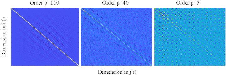
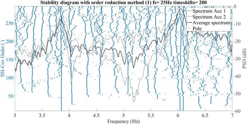
Fig. 2 shows the calculated results with the method presented in chapter 2, where the matrices ${\mathbf{U}}_p$ and ${\mathbf{V}}_p$ loss their orthogonality. Usually the stability diagram is cleared with different postprocessing methods (hard and soft validation criteria, modal transfer norm, ...) to enhance the interpretability of the results. [5] This was deliberately omitted to ensure the comparability of the two methods. The stable frequencies (4,039 Hz and 6,1157 Hz, [1]) are shown in the diagram by the vertical dotted line, but there are still many poles in the environment which could give the impression of a weaker excited natural frequency. These so-called mathematical poles or partially split modes make the interpretation of the results difficult, both manually and automatically.

Fig. 2Calculated Systempols without postprocessing (classic method 1) of a real 2DOF-system

The results of Fig. 3 were calculated with the method presented in this chapter, where the matrices stay orthogonal. If the diagrams resulting from the calculations are compared with each other, it is clearly shown that although mathematical poles were calculated, but these occur much more randomly and only actually existing natural frequencies form a continuous straight vertical line, which makes it much easier to interpret the stability diagram. Similar results can also be achieved with simulated data of a three-mass oscillator. Further studies will show which effects this calculation method with more random distributed poles have on the subsequent clustering regarding calculation time and precision.

4. Reconstructed shadow Hankel matrix for mode extraction

A further approach for calculation of clearly interpretable stability diagrams will be shown in this chapter. Based on a method used by Zhao and Jia described in [6] in the context of signal denoising and image processing for compressing images, the following equation Eq. (12) forms the necessary framework:

and $u_i\in {\mathbb{R}}^{p\times 1}$, $v_i\in {\mathbb{R}}^{p\times 1}$ are column vectors of the respective matrix.

Fig. 3Calculated Systempols without postprocessing (classic method 2) of a real 2DOF-system

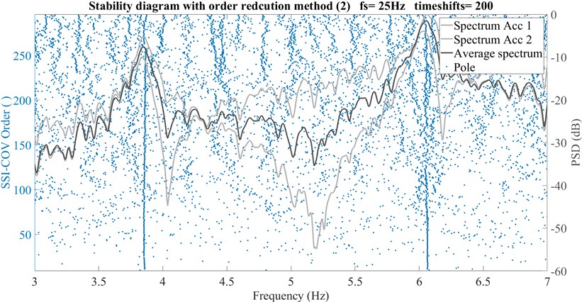
Fig. 43D-Stability plot of 3DOF simulated system and shadow Hankel matrix

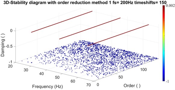
A natural frequency or a harmonic that is found in the recorded acceleration spectrum is shown by pairs of singular values. If a natural frequency or a region of interest in the singular value curve is identified, Eq. (12) allows the reconstruction of a reduced shadow Hankel matrix (${\mathbf{H}}_{0red}$), which is only reconstructed from the desired singular value pairs with the associated ${\mathbf{u}}_i$ and ${\mathbf{v}}_i$ vectors. The structure of the ${\mathbf{H}}_{0red}$ is like the original Hankel matrix ${\mathbf{H}}_0$, if enough singular pairs are selected but the absolute values are different for each cell compared between ${\mathbf{H}}_0$ and ${\mathbf{H}}_{0red}$. If the algorithm described in chapter 2 is now continued from Eq. (9) with the algorithm described in Eq. (12), the result for the data of the state space simulation of the accelerations of a 3 mass-spring-damper system including the first six singular values with the corresponding column vectors in two-dimensional space (i.e. order over frequency) is almost identical to the conventional calculation. If a third dimension (frequency, order and damping) is added, the advantage of this reduction is clearly visible. Without exception, all mathematical poles are now located in the range of negative damping. Fig. 4 with the help of this unambiguous allocation, all irrelevant poles can be removed. If, for instance, natural frequencies are known from previous analysis and can be assigned to the singular value pairs, this allows a very precise selective observation of individual frequencies. The shown eigenfrequencies and values for damping fit perfectly to the analytic data. Same results are obtained by use of data from the real 2-DOF System [1].

5. Summary and outlook of the accomplished work

The modifications of the classic SSI-COV algorithm presented here, favour the creation of clean stability diagrams. If the singular value decomposition is repeated for smaller Hankel matrices, the calculation effort increases and due to the decreasing dimensions of the matrices ${\mathbf{U}}_p$ and ${\mathbf{V}}_p$, the accuracy of pole estimation can also be reduced for lower calculation orders. However, as can be seen in Fig. 2 and Fig. 3, the interpretability of the stability diagrams is made much easier. The reconstruction of the Hankel matrix presented in chapter 3 leads to a loss of the typical Hankel structure, without interfering the SSI-COV algorithm. If the model order of the system is known, the reconstruction with the corresponding singular values allows an exact calculation of the system poles. All other mathematical poles fall out of the grid without application of hard or soft validation criteria due to the clearly implausible damping. Eq. (12) allows the removal of undesired natural frequencies or harmonics that are found in the acceleration spectrum due to the excitation. However, the lack of knowledge about the model order can be a problem in the application, as well as the fact that a reconstruction is done with too less pairs of singular values. There is a need for further research to transfer the results as shown in Fig. 4 to more complex and unknown systems in order to increase the degree of automation of the modal analysis.

References

-
Klein H. Development of a Test Stand and Measurement Concept for Vibration-Based Structural Health Monitoring Systems. Bachelor Thesis, University of Siegen, 2018.
Rainieri C., Fabbrocino G. Operational modal analysis of civil engineering structures. An introduction and guide for applications. Springer, New York, 2014.
Juang J., Pappa R. An eigensystem realization algorithm for modal parameter identification and model reduction. Journal of Guidance, Control and Dynamics, Vol. 8, Issue 5, 1985, p. 620-627.
Brincker R., Andersen P. Understanding stochastic subspace identification. Conference Proceedings: IMAC-XXIV: A Conference and Exposition on Structural Dynamics Society for Experimental Mechanics, 2006.
Reynders E., Houbrechts J., Roeck G. de Automated interpretation of stabilization diagrams. Modal Analysis Topics, Vol. 3, 2011, p. 189-201.
Zhao M.,Jia X. A novel strategy for signal denoising using reweighted SVD and its applications to fault feature enhancement of rotating machinery. Mechanical Systems and Signal Processing, Vol. 94, 2017, p. 129-147.
About this article