Temperature difference measurement with using two RTD sensors as example of evaluating uncertainty of a vector output quantity

1. Introduction

Temperature is the most frequently measured parameter in healthcare, industrial, air conditioning and ventilation, robotic and automotive applications [1], [2]. To know temperature or temperature difference with the right balance of accuracy, precision and repeatability is critical in many applications [3]. Commonly used in temperature measurement are resistance temperature detectors (RTDs) – precise metal components usually made of pure or almost pure platinum. The platinum sensor (e.g. Pt100) has a fully defined, repeatable and characterized resistance vs. temperature function. Therefore, RTD sensors are widely used in scientific and instrumentation applications. Moreover, many applications require multiple RTDs, so the interface and associated circuitry must also be appropriate for the application [4], [5].

Standard platinum RTD sensors (IEC 60751) operate in the range of –200 °C to + 800 °C. They are properly driven by a current or voltage source [6]. Their resistance is measured as a voltage across two terminals with an appropriate analog front-end (AFE) circuit, with the voltage reading it is linearized for the highest accuracy. Lead-wire-resistance compensation techniques are used.

The simultaneous temperature difference $t_D$ and average $t_{av}$ readings can be taken as an example of the multivariate measurement [7]. A Wheatstone bridge-circuit, classically supplied, can be used for measuring temperature, i.e. with one or two resistance temperature detectors (RTDs). It is widely presented in publication [8] where the values of limited errors and expanded uncertainties are calculated for a few variants of this circuit with the Class A and B industrial Pt100 sensors. However, this approach assumed that input and output measurands were uncorrelated. In this article the correlated measurands are considered.

Having transfer function of a bridge-circuit, the descriptive statistics which bases on evaluating uncertainty, can be performed. It is based on a vector method for determining uncertainty of multivariate indirect measurements, which is presented in Supplement 2 to the GUM Guide [9]. In this paper such approach is presented.

Propagation of measurement uncertainty using covariance matrix assumes that the input measurand is formulated by a random vector $\mathbf{X}={\left[X_1,X_2,\dots ,X_m\right]}^T$ and the output measurand by a random vector $\mathbf{Y}={\left[Y_1,Y_2,\dots ,Y_n\right]}^T$. The vectors of dimensions $m$ and $n$ represent the multi-dimensional distributions of $\mathbf{X}$ and $\mathbf{Y}$. If $f$ is a linear operator, then $n\le m$. The relation between them is presented as a generalized equation [10]:

where $f$ describes the system equation as a function of the input quantities, while $f\text{'}$ is a function of the uncorrelated subsystems. Vector $\mathbf{h}$ contains the uncertainties of every subsystem $\mathbf{h}=[{{\mathbf{h}}_1^T,\dots ,{\mathbf{h}}_K^T]}^T$. Symbol $K$ represents the number of subsystems [11].

The relation between covariance matrices ${\mathbf{c}}_{\mathbf{X}}$, ${\mathbf{c}}_{\mathbf{Y}}$ of the output measurand $\mathbf{Y}$ and input measurand $\mathbf{X}$ is expressed as:

where $\mathbf{S}\equiv \partial \mathbf{Y}/\partial \mathbf{X}$ is the matrix of sensitivity coefficients [12]. The model Eq. (2) is true if it is either linear or can be linearized in the working point using a Taylor series. Usually, the uncertainties for the input parameters are small. Another assumption is that the probability density functions (PDFs) should be symmetric and common.

A covariance matrix c and a correlation matrix $\mathbf{K}$ are defined by:

where $\mathbf{\sigma }$ is the diagonal matrix of standard deviations [10].

2. Average and difference temperature measurement – circuits, transfer functions, uncertainty

There are many designs of analog front-end circuits for RTDs measurement. In Fig. 1(a) classical Wheatstone bridge-circuit is presented. Another circuit (Fig. 1(b)) differs from the previous one, i.e. output voltages are proportional to a difference and a sum of temperatures $t_1$, $t_2$, starting with the initial temperature $t_0$. This circuit is the alternative to the classical bridge-circuit. Both circuits were described in previous articles of authors [8], [13]. Below, the uncertainty propagation will be expressed using model Eq. (2).

Fig. 1a) The classical and unconventional, b) bridge-circuits as resistance to voltage converters, the resistances R1 and R2 represent two RTDs

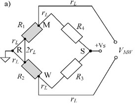
Two transfer resistances $r_{AB}=f_1\left(t_D\right)$, $r_{CD}=f_2\left(t_{av}\right)$ of the bridge-circuit depend on the resistances $R_1$…$R_4$ in different way (assuming that constant currents $J$ are equal):

where: $\mathrm{\Sigma }{R}_i=R_1+R_2+R_3+R_4$, lead resistances $r_L\ll R_1,R_2,R_3,R_4$.

An input matrix ${\mathbf{c}}_{\mathbf{X}}$ contains only variances (squared uncertainties) because it is assumed that the input variables are uncorrelated and normally distributed:

The sensitivity matrix is as follows:

The output variance-covariance matrix ${\mathbf{c}}_{\mathbf{Y}}$ is a two-dimensional quantity:

This matrix can be depicted by an ellipse in the plane [9]. It is the horizontal intersection curve of the Gaussian probability surface with a plane at the level of its inflection point.

Having the covariance, the Pearson’s correlation coefficient is defined:

Its value is within the range from –1 to 1. Below, the dependence of covariance from the bridge resistances Eqs. (9-10) and their squared uncertainties Eqs. (11-12) are presented:

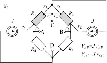
If there are two RTDs in the bridge-circuit then $R_i=R_0+\mathrm{\Delta }{R}_i$ (for $i=$1, 2) and $R_i=R_0$ (for $i=$3, 4), when $R_0$ is nominal resistance (e.g. 100 Ω). According to IEC 60751 standard the operating limits of a Pt100 sensor $R_i$ can be within the range from 81.48 to 390.48 Ω. This corresponds to the temperature range from –200 to +850 °C. In Fig. 2 the transfer resistances Eq. (4) are presented in a function of $\mathrm{\Delta }{R}_1=2\mathrm{\Delta }{R}_2$ within the range of from –80 to +80 Ω.

Also, assume that there are two uncertainties: of sensors ${\sigma }_{R1}={\sigma }_{R2}={\sigma }_{Sen}$ and of resistors ${\sigma }_{R3}={\sigma }_{R4}={\sigma }_{Res}$. In this case output covariance and uncertainties are as follows:

Fig. 2Dependence of the transfer resistances on the change in resistance when ΔR1=2ΔR2 t1=2t2. The temperature difference tD=t1-t2 range is limited by nonlinearity of the transfer resistance rAB

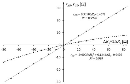
Fig. 3Dependence of the Pearson’s correlation coefficient on the change in resistance when ΔR1=-ΔR2, different relationships of σSen and σRes are assumed. When σSen≫σRes the correlation (positive and negative) is the highest

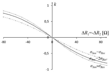
Fig. 4Dependence of the Pearson’s correlation coefficient on the change in resistance when ΔR1=2ΔR2. This coefficient does not exceed ±0.4

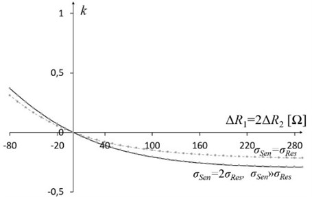
Fig. 3 presents dependence of correlation coefficient on the change in resistance when $\mathrm{\Delta }{R}_1=-\mathrm{\Delta }{R}_2$. Fig. 4 depicts it for $\mathrm{\Delta }{R}_1=2\mathrm{\Delta }{R}_2$. When $\mathrm{\Delta }{R}_1=\mathrm{\Delta }{R}_2$ correlation coefficient $k$ is equal to 0.

3. Conclusions

The application shows the usage of variance-covariance matrix for estimating uncertainties of two transfer resistances ($r_{AB}$, $r_{CD}$) of the circuit model. Using Eqs. (4-12) the novel description of the brigde-circuit was created. It develops a wider discussion on the resistance-to-voltage converters and their applications. The maximum nonlinearity error of transfer resistance $r_{AB}$ is 3 % when temperature $t_1$ varies from –200 to 200 °C and temperature $t_2$ is half of $t_1$ (Fig. 2). Fig. 3 and Fig. 4 depict two variants of relationship between the increments of sensors’ resistances when the Pearson’s correlation coefficient is different than 0. It shows that both measurement result values should contain standard uncertainties as well as a correlation factor.