A deep learning-based approach for automatic detection of concrete cracks below the waterline

2.1. Mathematical models for the sea surface

Different propagation events are influenced by the light depending on the topography of the seabed and streamer depth. The scenarios are used to anticipate how the optical effects might impact the underwater pictures by feeding them into a model for underwater wave propagation.

Wave models are increasingly employed in a variety of coastal areas to research and predict wave conditions. They can be structured using both wave action models (also known as phase averaging models) and momentum models (or phase resolving models). The third generation of phase averaging models is used in a wider range of applications. Many advanced professional engineering applications, such as flow simulations and wave modeling, are available through commercially available software. Not all prepared and accessible models, meanwhile, are adjusted to the photos used to identify underwater cracks.

The basis for modeling ocean waves is the linear (or small-amplitude) wave theory of Airy [4], which is commonly used in marine engineering and computer graphics (Peachey [5]. It describes sinusoidal waves, which are connected to clear skies. Trochoid models made by von Gerstner [6] and by Fournier and Reeves [7] were used to make their description more accurate (Rankine) [8]. Random waves are produced by combining numerous waves and applying an equation to a 2D surface. Another method is the 2D inverse discrete Fourier transform, which has been used by Premože and Ashikhmin [9], Mastin et al. [10], Tessendorf [11] and others.

Oceanographers are more concerned about wave energy than amplitude. They do this by using a different type of spectrum, $S\left(w\right)$, sometimes referred to as a wave spectrum or a frequency energy spectrum, which offers information on the distribution of wave energy as a continuous function of frequency [12]. Taking wind speed into consideration, Pierson and Moskowitz [13] developed a formula for the sea. However, the JONSWAP spectrum has been shown to be more appropriate for a fetch-limited sea with rising waves (Hasselmann et al.) [14]:

where ${\omega }_p$ is the frequency of the peak of the spectrum. Usual value for ${\omega }_p$ is equal to ${\omega }_p=0.855g/U_{10}$, where $U_{10}$ is the speed of wind at the height of 10 meters above the sea surface. Here $\gamma$ is the peak enhancement factor, parameter $\sigma$ depicts the width of the peak. The values for the parameters in this spectrum equation are:

where $F$ is the fetch in meters, usually $\gamma =$ 3.3, but can vary from 1 to 7, and:

Since the fetch is an essential part of the description of the sea state, we use the JONSWAP spectrum rather than the Pierson-Moskowitz one.

The equation $S\left(\omega ,\theta \right)=S_J\left(\omega \right)G\left(\omega ,\theta \right)$ denotes the directional spectrum of sea waves, sometimes referred to as the directional spectrum function, which is used to describe the characteristics of the wave direction, where $G\left(\omega ,\theta \right)$:

This article employs the directional extension feature suggested by the stereo wave observation project (SWOP) [15].

The Double Summation Model may express the sea surface elevation $H\left(x,y,t\right)$ [16]:

where $a_{ij}$ is the wave amplitude of frequency $i$ and directional angle $j$. ${\theta }_j$ is extending directional angle of the wave $\left(0<\theta \le 2\pi \right)$, ${\omega }_i$ is example frequency within the frequency division range. $k_i$ is the wave number and the value is equal to $k_i={\omega }_i^2/g$, ${\epsilon }_{ij}$ is the random initial phase angle $\left(0\le {\epsilon }_{ij}<2\pi \right)$.

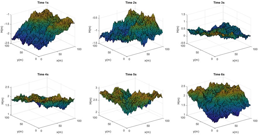
MATLAB can simulate 3D ocean waves since it has a large library for mathematical calculational and a variety of 3D graphic processing options. By looking at the ideal diagram of the JONSWAP spectrum and SWOP directional extension function under $U_{10}=$ 20 m/s, we determined the appropriate range of angular frequency and direction angle for equal division and created a three-dimensional sea surface wave model at a specific time over a specified sea area. An angular frequency in the [0.01, 4] range was used to numerically replicate the average frequency via frequency equal division method. With $N$ and $M$ equal to 35, $\mathrm{\Delta }\omega =$ 0.114 rad/s, $\mathrm{\Delta }\theta =$ 0.0898 rad, we divided the direction angle of $\left[-\pi /2,\pi /2\right]$. The Fig. 1 provides an illustration of the computation results over a period of 6 seconds.

Fig. 1Mathematical models of illustrations of sea surface at different times

2.2. Augmentation of the dataset by optical underwater effects

For realistic representations of water, proper control of the interaction between the water surface and light is essential. This realism may be achieved by computing reflections and refractions and using the Fresnel equations to calculate the intensity of the refracted and reflected light beams. Another important subject is underwater light absorption, which includes how light behaves as it passes through water.

Fig. 2Aspects of reflection of lights due at a point due to the surface undulations.

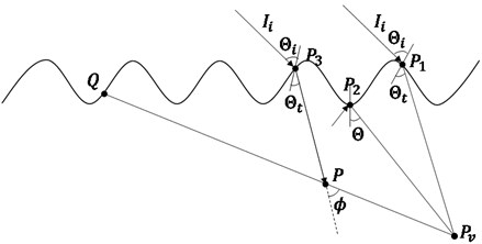
We describe how to determine how much light is coming into the viewpoint. One must account for the light scattering brought on by water droplets when illustrating light shafts. According to [17], the equation below calculates the quantity of light $I_v\left(\lambda \right)$ that goes from point $Q$ on the water’s surface to perspective $I_v$ when one is observing from underwater:

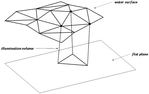
where $L$ is the distance between $P_{v}Q$, $l$ is the distance between $P{P}_v$, $c\left(\lambda \right)$ represents the attenuation coefficient of light within water while the intensity of light dispersed at point $P$ is indicated by $I_P$ (see Fig. 2). The whole technique of the rendering optical effects with graphics hardware is presented in [18] related to the generation of illumination volumes (see Fig. 3).

Fig. 3Generation of illumination volumes

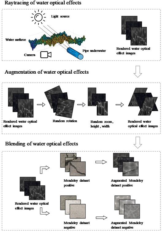
We provide a technique for producing optical effects underwater. In order to start, we’ll assume that the water’s surface is level. We identify the refraction vector of the sun. Second, we develop a texture that is a representation of depth as seen through the light's lens. The light is coming from the sun in a particular direction after it has been refracted. The third phase involves rendering a scene from the eye’s perspective (see Fig. 4). All the steps were completed with the Blender program. We compare the values of the two textures in order to determine if a pixel is shadowed or not.

We will use the 40,000 images of surfaces with and without concrete cracks from Ozgenel’s released data set of concrete crack pictures [19]. The network is trained using a collection of “Positive” and “Negative” images with a resolution of 227×227, and its accuracy is evaluated using a smaller set of test images. A virtual optical environment is used to recreate an image dataset with underwater optical effects. Using Blender’s Cycles, 60 realistic underwater caustic effects were produced, that represent the optical effects of moving water surface and ripples in time.

A separate optical water effect mask is made for each image in the 40,000 image of the Mendeley Concrete Crack Photos for Classification collection. We employed modifications like random rotation, random zoom, height, width, and shear to make 40,000 distinct optical water effect masks.

In order to improve concrete crack images, image superposition techniques are utilized to merge two images (a concrete surface and a water optical effect mask). This is accomplished by employing several blending techniques. This procedure is used over the whole data set of 40,000 photographs (once for images with and once for images without cracks). All the processes of the image augmentation are presented in Fig. 4.

Fig. 4Different steps of incorporating underwater optical effects on concrete surface images