Abstract
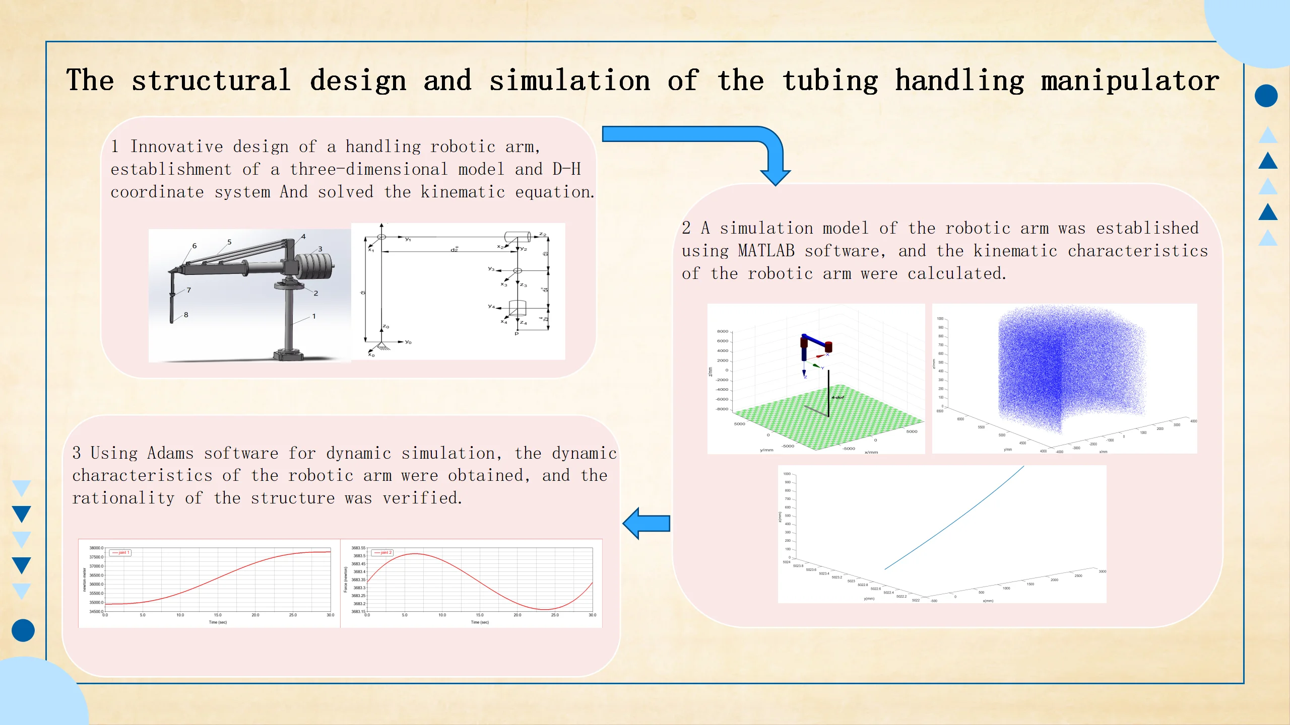
The size of the oil pipes in the factory is relatively large, making them inconvenient to handle. There are few existing oil pipe handling devices, and a 2P2R four degree of freedom manipulator device has been innovatively designed to complete the oil pipe handling work. First, the three-dimensional model of the manipulator was established using SolidWorks software, and then the improved D-H method was used to carry out the kinematics modeling of the manipulator system, and the forward and Inverse kinematics equations were derived. Then, the MATLAB software was used to carry out the kinematics analysis of the manipulator, and the manipulator workspace was calculated. The movement trajectory, as well as the displacement, speed, and acceleration curves under the trajectory were obtained using the fifth order Polynomial interpolation method, Finally, the 3D model was imported into Adams software, and an Adams virtual prototype was established for dynamic analysis. The force and torque curves of each joint were obtained, laying the foundation for further design and research in the future.
Highlights
- Novel mechanical arm structure
- Established kinematic equations and verified the good kinematic performance of the robotic arm
- Dynamic simulation was conducted to verify the rationality of the structure
1. Introduction
In today 's society with the in-depth development of artificial intelligence, robotic arms play an important role in many fields. In the factory, the traditional manual work cannot meet the actual needs of social production [1]. The mechanical arm works step by step according to the preset instructions, and there is almost no error, which not only greatly improves the production efficiency, but also solves the problem of difficult employment in enterprises [2].
Because the manipulator handling process is to adsorb the tubing from the ground and then move it to the steel frame, a set of four degrees of freedom manipulator system is designed to meet the needs of the whole task. The four degrees of freedom are two translation pairs and two rotation pairs, which are an underactuated cylindrical coordinate manipulator [3]. The improved D-H method is used to establish the forward kinematics equation, and the geometric method is used to establish the inverse kinematics equation. And then the kinematics and dynamics simulation of the manipulator is carried out to verify the correctness of the manipulator model.
2. The establishment of three-dimensional model and D-H coordinate system
SolidWorks software is used to establish the three-dimensional model of each part and assemble it into a physical diagram, as shown in Fig. 1, where 1 – unable adjustment base; 2 –bottom rotary joint; 3 – counterbalance; 4 – connecting piece; 5 – diagonal tie; 6 – radial translation joint; 7 – terminal rotary joint; 8 – vertical translation joint.
The length of the handling tubing is about 10 m, so the design size of the whole manipulator is large. In order to reduce the weight of the system, aluminum alloy will be used as the main material. The bottom rotary joint controls the whole manipulator to rotate around the base, and the range of motion is –60°-60°. The radial translation joint uses a linear hydraulic cylinder to control the radial expansion motion of the manipulator, and the range of motion is 0-1400 mm. The end rotary joint controls the end of the manipulator to rotate, and the range of motion is –90°-90°. The vertical translation joint controls the translation motion of the end in the vertical direction, and the range of motion is –1200-0 mm.
The manipulator system controls the end of the manipulator to complete the expected complex action by inputting different instructions to each joint. The trajectory of the end of the manipulator is affected by the coordinates and pose of each joint of the manipulator [4]. In this paper, the improved D-H method is used to establish the D-H coordinate system, and the forward and reverse solutions of each joint of the manipulator are obtained [5-6]. The coordinates of the four-degree-of-freedom manipulator in the optimized and improved Cartesian space are set as shown in Fig. 2.
Fig. 1Three-dimensional model
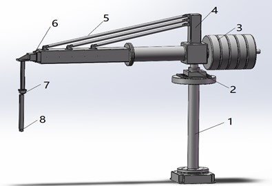
Fig. 2D-H coordinate system
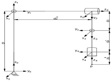
The manipulator in this paper is mainly composed of two rotating pairs and two translation pairs. After establishing the joint coordinate system, the D-H parameters of the manipulator can be determined according to the adjacent joint coordinate system [7]. The parameters , , , of the coordinate system established by the improved D-H method, and respectively represent the length of the connecting rod, the torsion angle, the offset of the connecting rod and the joint angle. As shown in Fig. 2, the end point of the manipulator is , and the distance from the point to the coordinate system is. The D-H parameters of each link of the manipulator are shown in Table 1.
Table 1D-H parameters
Range of motion | |||||
1 | 0 | 0 | –60°-60° | ||
2 | –90° | 0 | 0 | 0-1400 mm | |
3 | –90° | 0 | –90°-90° | ||
4 | 0 | 0 | 0 | –1200-0 mm | |
Note: Variables with *= 4695 mm, = 1313 mm | |||||
3. The establishment of kinematics model direct kinematics solution
The forward kinematics problem is to solve the pose of the end of the manipulator when the joint variables are known [8]. Starting from the coordinate system {0}, the pose transformation matrix from to is obtained in turn, and the transformation matrix between the two adjacent links of the manipulator is:
The transformation matrix of adjacent joints can be obtained by substituting the parameters in the D-H parameter table into the Eq. (1). The transformation matrix of coordinate system {0}-{4} can be obtained by multiplying the obtained matrix in turn. And the distance of the end point p in the coordinate system is , then its transformation matrix to the coordinate system is:
The meanings of , , , are respectively , , , .
The transformation matrix obtained by Eq. (2) is a 4×4 matrix, which can determine the pose of the manipulator. The 3×3 matrix on the left represents the pose of the manipulator, and the 3×1 matrix on the right represents the position of the manipulator. It can be seen that the position of the manipulator is only related to the rotation angle of the two joints and . The position of the end of the manipulator is related to the three variables of , and , but not to .
4. Inverse kinematics solution
When solving the inverse kinematics, it is usually very difficult to use the algebraic method to solve the forward kinematics solution. Therefore, this paper uses the geometric method to solve the inverse kinematics of the manipulator joint. The coordinates of the end point in the coordinate system are (. According to the established D-H coordinate system, it can be known from the geometric relationship:
The angle between the tubing on the ground and the coordinate axis is set to be . In order to facilitate the subsequent calculation work, the initial position of the end point of the manipulator is set at (0, 5023, 50), and the value of each joint variable can be obtained:
According to the Eq. (6-9), the variables of each joint of the manipulator can be solved under the condition that the pose of the end of the manipulator is known. Among them, is the function of arctangent value in MATLAB.
5. Simulation
5.1. Workspace analysis
The workspace of the robot is a set of points that can be reached at the end of the manipulator, which is determined by the size structure and joint motion range of the manipulator [9]. The Monte Carlo method is a robot workspace analysis method based on random probability [10]. Using this method, the workspace of the manipulator can be solved more accurately, but the premise of using this method is to ensure that the joint motion range of the modeling and the actual model is consistent. Using MATLAB software, the simulation model is first established as shown in Fig. 3(a) below, and then the workspace is simulated. The results are shown in Fig. 3(b). It can be seen that the workspace of the four-degree-of-freedom manipulator is roughly in a sector area, which meets the work requirements.
Fig. 3Manipulator simulation model and workspace
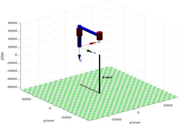
a) Manipulator simulation model
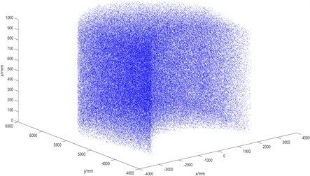
b) Manipulator workspace
5.2. Simulation analysis of trajectory planning based on MATLAB
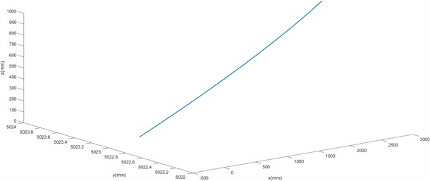
The trajectory of the manipulator is the trajectory of the end of the manipulator moving from the starting point to the end point in space, which can be expressed by the displacement, velocity and acceleration of each joint [11]. The actual working requirements of the four-degree-of-freedom manipulator will make the end of the manipulator move from the starting point (0, 5023, 50) to the end point (–2900, 5023, 1000). The ikunc function of MATLAB robot toolbox is used to solve the coordinates of each joint, and the trajectory is formed by 5 polynomial interpolation. This trajectory can effectively avoid the problem of excessive acceleration caused by the sudden change of speed at the starting point and the end point. The trajectory curve is shown in Fig. 4. The end of the manipulator can move smoothly in space and complete the work.
Fig. 4End trajectory of mechanical arm
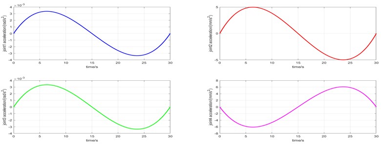
The plot function is used to draw the displacement, velocity and acceleration curves of each joint with time. Because it is a 2P2R manipulator, the motion types of each joint are different. Therefore, the curves of each joint are drawn separately. The curves are shown in Figs. 5-7. In the following figure, joint 1 is the bottom rotating joint in Fig. 1, joint 2 is the radial translation joint, joint 3 is the end rotating joint, and joint 4 is the vertical translation joint.
It can be seen from Fig. 5-7 that during the movement of the end of the manipulator from the starting point (0, 5023, 50) to the end point (–2900, 5023, 1000), joint 1 changes from 0 rad to /6 rad, joint 2 changes from 0 mm to 777 mm, joint 3 changes from 0 rad to /6 rad, and joint 4 changes from 0 mm to-950 mm. The velocity of each joint reaches the maximum at 15 s, and the acceleration reaches the maximum at 6 seconds and 25 seconds. In the process of movement, the displacement, velocity and acceleration curves of each joint correspond to each other and are smooth and stable. There is no sharp increase or decrease in velocity and acceleration, which indicates that the structural design of the manipulator is reasonable. The manipulator can reach the specified position continuously and smoothly according to the working requirements.
Fig. 5Displacement curve of each joint
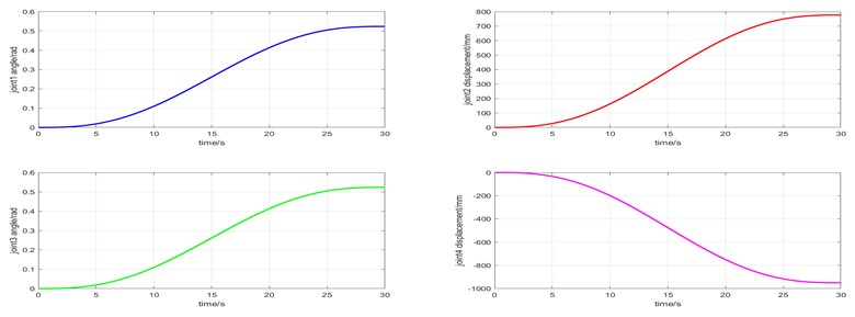
Fig. 6Velocity curve of each joint
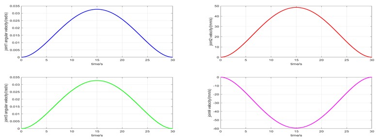
Fig. 7Acceleration curve of each joint
5.3. Dynamics analysis based on Adams
The three-dimensional model of the four-degree-of-freedom manipulator is imported into Adams software. Firstly, the simulation conditions of gravity and unit are set up, the material of the manipulator is modified to aluminum alloy, and then the constraint conditions are defined. The starting point coordinates (0, 5023, 50) and the end point (–2900, 5023, 1000) are substituted into the Eq. (12-15) to solve the value of the four joint variables, and then the rotation drive is added at the joint 1 and joint 3, and the translation drive is added at the joint 2 and joint 4. The drive at each joint is set as shown in Table 2. The range of motion of the drive function in each joint is determined by the value of the solved joint variables.
Table 2Joint drive function
Joint | Drive function |
Joint 1 | STEP5(time,0,0,30,-30d) |
Joint 2 | STEP5(time,0,0,30,-777) |
Joint 3 | STEP5(time,0,0,30,30d) |
Joint 4 | STEP5(time,0,0,30,950) |
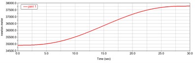
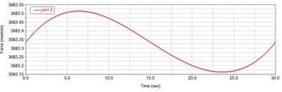
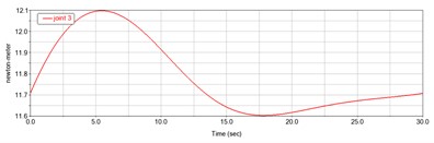
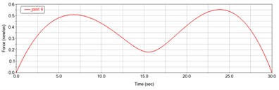
The simulation time is set to 30 s, and the number of simulation steps is 1000 steps. The simulation results of each joint force and torque are shown in Fig. 8.
It can be seen from Fig. 8 above that the torque of joint 1 gradually increases with time, the maximum value of joint 2 force appears in about 6 seconds, the maximum value of joint 3 torque also appears in about 6 seconds, and the maximum value of joint 4 force appears in about 24 seconds, which is the key point to be considered in the subsequent selection of motor. The four joints have peaks in the simulation process in about 6 seconds or 25 seconds, which is consistent with the acceleration curve of each joint in Fig. 6, and the changes of force and torque are relatively gentle. It is verified that the dynamic performance of the manipulator is better.
Fig. 8Force and torque curves of each joint
a) Joint 1 torque curve
b) Joint 2 force curve
c) Joint 3 torque curve
d) Joint 4 force curve
6. Conclusions
1) In this paper, a 2P2R four-degree-of-freedom manipulator is designed to replace the manual handling of long and heavy metal tubing. The three-dimensional model of the manipulator is established. The forward and inverse kinematics equations of the manipulator are derived by using the improved D-H method, and the correspondence between the joint variables and the world coordinates of the manipulator in space is verified.
2) Using MATLAB software, according to the forward and inverse kinematics equations, the trajectory planning analysis is carried out by using the quintic polynomial interpolation method. The working space of the manipulator, the end motion trajectory and the displacement, velocity and acceleration curves of each joint are obtained, which verifies the reliability of the structural design and the correctness of the kinematics equation.
3) The three-dimensional model is imported into Adams software for dynamic analysis, and the force and torque curves of each joint are obtained. The rationality of the manipulator design is further verified, which provides an important basis for the selection of key components such as motors and reducers.
References
-
C. Siyu, “Design of a six-degree-of-freedom robotic arm sorting system based on machine vision,” Internal Combustion Engines and Accessories, Vol. 11, pp. 43–45, 2022.
-
W. Jia, Y. Tian, R. Luo, Z. Zhang, J. Lian, and Y. Zheng, “Detection and segmentation of overlapped fruits based on optimized mask R-CNN application in apple harvesting robot,” Computers and Electronics in Agriculture, Vol. 172, p. 105380, May 2020, https://doi.org/10.1016/j.compag.2020.105380
-
L. Lin, W. Juan, and W. S. Yan, “Structural design and kinematics analysis of 6R explosive ordnance disposal manipulator based on hydraulic motor drive,” Machine Tools and Hydraulics, Vol. 47, No. 23, pp. 64–68, 2019.
-
Z. F. Jun et al., “Considering the fuzzy control of the end pose accuracy of the joint clearance manipulator,” Manufacturing Technology and Machine Tool, Vol. 2020, No. 6, pp. 148–154, 2020.
-
Z. F. Lin, Y. Y. Long, and L. Guang, “Research on singular trajectory method for inverse kinematics of space 3R manipulator,” Mechanical Science and Technology, Vol. 38, No. 3, pp. 365–372, 2019.
-
L. G. Long et al., “Forward kinematics and workspace analysis of screw theory for seven-degree-of-freedom dual-arm robot,” Mechanical Science and Technology, Vol. 38, No. 5, pp. 704–712, 2019.
-
Y. Sheng, W. H. Yu, Y. He, and T. Hui, “4-DOF modular mobile manipulator modeling and kinematics analysis,” Modern Electronic Technology, Vol. 34, No. 15, pp. 204–207, 2011.
-
C. L. Gang, P. X. Liang, and X. X. Wen, “Trajectory planning and simulation of planar three-degree-of-freedom manipulator,” Tool Technology, Vol. 45, No. 9, pp. 26–30, 2011.
-
W. G. Wei et al., “Design and kinematics simulation of a continuous line driven manipulator,” Mechanical Transmission, Vol. 43, No. 11, pp. 32–38, 2019.
-
W. Jie et al., “Kinematics analysis and simulation of a serial robot for fruit and vegetable harvesting,” Manufacturing Automation, Vol. 45, No. 5, pp. 50–54, 2023.
-
Zhang Chang, Wu Yu-Qiang, “Kinematics modeling and simulation of six degrees of freedom manipulator based on P-rob,” Packaging Engineering, Vol. 41, No. 11, pp. 166–173, 2020.
About this article

The authors have not disclosed any funding.
The datasets generated during and/or analyzed during the current study are available from the corresponding author on reasonable request.
The authors declare that they have no conflict of interest.
