Trajectory planning and control algorithm of industrial robot manipulator

Liu, Jing

doi:10.21595/jve.2023.23274

Journal of Vibroengineering

Browse Journal

Submit article

Published: 08 August 2023

Check for updates

Trajectory planning and control algorithm of industrial robot manipulator

Jing Liu¹

¹Intelligent Manufacturing College, Chongqing Creation Vocational College, Chongqing, 402160, China

Cite the article Download PDF

Downloads 245

Abstract

As the industrial robot task becomes more complex, the difficulty of trajectory planning and tracking control of manipulator is gradually increasing. To minimize the vibration during the manipulator motion and improve the planning accuracy, the method of quintic polynomial combined with non-uniform B-spline interpolation is studied for joint space (JS) planning. The trajectory tracking system is easily affected by friction nonlinearity and parameters. So a JS trajectory tracking controller based on based on fuzzy neural network (FNN) is designed. Through simulation experiments, the curve obtained by the planning method studied is smoother and the planning error is minimum. The maximum position error is 0.09 rad, and the speed error is not more than 0.1 rad/s. The controller performance test results under different parameters show that the $\hat{W}$ , $\hat{c}$ , $\hat{κ}$ parameter in FNN can be adjusted in real time, and the value will not affect the performance of the controller. The fluctuation range of trajectory error of different joints is within ±0.2×10^-5rad, which indicates that the performance of AFNNC controller studied is better. And its response time is the shortest and its robustness is better when the load changes suddenly.

1. Introduction

With the accelerated pace of social development, industrial robots play an increasingly important role in the manufacturing industry. The work efficiency can be effectively improved by industrial robots. Human losses and economic costs can be reduced. And a strong guarantee can be provided for the development of the entire industry [1]. Some actions of human arm can be imitated by robot arm. Robot arm is an automatic operating device that grabs and transports objects or operating tools with fixed procedures. Not only human command can be accepted, but also pre-programmed procedures can be run [2]. Because of its high safety, tirelessness and other advantages, human beings can be liberated by using robot arm from the dangerous and fatigue environment. While providing convenience for human life, social production can be improved, and the productivity can be promoted [3]. For industrial production, the manipulator is widely used in arc welding, spraying and other tasks. At present, with the acceleration of the pace of social development, industrial robots have made considerable progress in automation and intelligence, which has played a great role in promoting the development of robot technology. The rapid development of robot technology not only provides convenience for people’s life, but also provides direct economic benefits for the whole country, and also promotes the development of the whole science and technology. At present, the industrial robots around the world have undergone three generations of upgrading and transformation, and their performance and accuracy have been greatly improved. However, in some complex and fine industrial tasks, higher requirements have been put forward for the tracking accuracy of the given robotic arm trajectory throughout the entire working process [4].

With industry developing, the tasks completed by the manipulator are more complex, and the difficulty of trajectory planning and tracking control is increased. Aiming at the problems of bounded uncertainty and large initial error in manipulator trajectory planning of free-floating space robots with both arms, a wrist trajectory planning method is proposed by Yan W's research team by using time-fixed characteristics to eliminate errors caused by singularity. A terminal controller is also designed which can achieve new low buffeting and global non-singularity through state approach Angle and switching sliding mode. The simulation test after the combination of the two shows that the accuracy of wrist trajectory planning can be improved by this controller. And the trajectory tracking accuracy can be improved to nanometer level. The research scheme is feasible [5]. To enable robots to complete assigned tasks and avoid collision with obstacles, motion planning through the joint of both arms has been studied by Ni S and other scholars. In order to avoid obstacles, the trajectory planning problem is transformed into a trajectory optimization problem, and a particle swarm optimization algorithm is used to find the optimal trajectory of the robot. The kinematic singularity problem can be avoided by the proposed planning method more efficiently. The task completion time could be saved and the work efficiency can be improved by the optimal trajectory [6]. A graph-based path search algorithm was proposed by Kaljaca D and other researchers for the trajectory planning of the pruning robot. This algorithm mainly performed function interpolation in JS to achieve path search. Through model simulation test, the results showed that the problem of trajectory error caused by excessive arm movement could be avoided by this algorithm. And the positioning accuracy of cutting blade was higher than 90 %. The actual test results showed that the robot trimming error was within mm [7]. When facing the path restriction problem, a time optimal path planning method that takes into account the optimal path search was proposed by Yu X. and his members. A interpolation algorithm was used to derive the motion curve equation of the joint, and the motion time and path points can be optimized by genetic algorithm. The optimal motion path of the manipulator could be obtained by this method [8].

Rich researches on the trajectory tracking of manipulator was carried out. Trajectory tracking control analysis was carried out by Hu Q's research team for the manipulator with three degrees of freedom. An adaptive controller was studied and designed, and the kinematics equation was used to study the control strategy of multi-level switching. The tracking control accuracy of the control strategy was higher than 90 %, which verified the high accuracy of the method [9]. The robot was expected to achieve accurate trajectory tracking. The use of radial basis function neural networks was studied by Zhang Y. et al to approximate the unknown, and a motion controller was designed. Through test, there were fewer unknown parameters, and the deviation between the robot motion trajectory obtained and the actual curve was small [10]. The trajectory control of the extension motion of the manipulator was analyzed by Uno Y's research team. A trajectory control scheme was designed by introducing differential feedback. With the desired trajectory, the trajectory of the manipulator could be modified by this scheme and the goal of convergence could be achieved. The trajectory convergence could be completed by this method in 10 iterations. Compared with other methods, this scheme was more flexible and applicable to many situations [11]. The original control algorithm of the surgical robot needed to be relearned when the target changed. So based on convolution neural network a low delay control strategy was proposed by Tian X. and other scholars by designing the vision layer and control layer of neural network. The motion trajectory of the manipulator could be controlled effectively, and the minimally invasive surgery could be completed accurately [12]. A general strategy framework was designed by Xia J. and other researchers for robot motion control, which mainly involved track tracking, obstacle avoidance, track analysis and other modules. According to the experimental test results, the feasibility of robot motion trajectory could be evaluated quickly by the strategy framework, and the trajectory tracking efficiency and accuracy were better [13].

Through a statement of the achievements of domestic and foreign researchers, it was found that the task of the manipulator is becoming increasingly complex. And there was an increasing demand for trajectory planning and real-time trajectory tracking. Most of the previous research were focused on the industrial robots’ performance improvement in terms of working efficiency, trimming error and route planning. But there is still a large room for improvement in the control accuracy, and the combination of intelligent algorithms is not deep enough. In the face of these requirements, the method of 5-time non-uniform B-spline interpolation is studied in this study for trajectory planning in JS. In order to improve the trajectory tracking accuracy of industrial robots, a tracking controller based on FNN is proposed innovatively in this study to solve the multiple constraints and large tracking errors in the tracking control system. And it is expected that it can plan the trajectory of the manipulator more accurately.

2. Research on trajectory planning and control method of manipulator JS

2.1. JS trajectory planning based on quintic non-uniform B-spline interpolation

In the actual operation of the industrial robot, the actual motion trajectory of its manipulator needs to be consistent with the expected trajectory [3, 14]. During manipulator motion, the speed, displacement, acceleration and other variables of each joint will change. Variable planning is crucial to achieve consistent trajectory [15]. When the robot manipulator trajectory's starting and ending point is determined, the displacement of each joint in JS can be inversely calculated by using the inverse kinematics knowledge. According to the required speed, acceleration and other parameter values, the method of quintic polynomial combined with non-uniform B-spline interpolation is studied to obtain the corresponding joint trajectory curve. The trajectory planning process in JS is shown in Fig. 1. For each joint, velocity and acceleration’s time function can be obtained by successively deriving the quintic polynomial of the curve. The non-uniform B-spline interpolation curve defined by the control vertices is analyzed. And the known parameters are substituted to solve the control vertices of the non-uniform B-spline interpolation curve. The velocity and acceleration curves of the robot's motion trajectory can be obtained by deriving the control vertices.

Fig. 1Trajectory planning process in JS

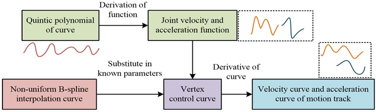
In trajectory planning, the curve segment between two nodes is generated by quintic polynomial fitting, and the whole curve is composed of multiple sets of quintic polynomials. The quintic polynomial function contains six unknown coefficients, and Eq. (1) is the expression:

1

θ (t) = a_{0} + a_{1} t + a_{2} t^{2} + a_{3} t^{3} + a_{4} t^{4} + a_{5} t^{5},

where, $a_{*}$ represents the acceleration of each joint. $θ (t)$ is the function of each joint with respect to time $t$ . The first and second order derivatives of time are performed for Eq. (1). The function formula (2) of velocity, acceleration and time $t$ of each joint can be obtained:

2

\{\begin{array}{l} 3 a_{3} t^{2} + 2 a_{2} t + 5 a_{5} t^{4} + 4 a_{4} t^{3} + a_{1} = \dot{θ} (t), \\ 12 a_{4} t^{2} + 6 a_{3} t + 20 a_{5} t^{3} + 2 a_{2} = \ddot{θ} (t), \end{array}

where, $\dot{θ} (t)$ and $\ddot{θ} (t)$ is the functional expressions of the first and second derivative respectively. The angular displacements $θ_{0}$ and $θ_{f}$ corresponding to the start time $t_{0}$ and the end time $t_{f}$ are known. The second-order continuity is satisfied, and the constraint conditions of Eq. (3) are satisfied:

3

\begin{array}{l} \{\begin{array}{l} θ (0) = θ_{0}, \\ θ (t_{f}) = θ_{f}, \end{array} & \begin{array}{l} \dot{θ} (0) = {\dot{θ}}_{0}, \\ \dot{θ} (t_{f}) = {\dot{θ}}_{f}, \end{array} & \begin{array}{l} \ddot{θ} (0) = {\ddot{θ}}_{0}, \\ \ddot{θ} (t_{f}) = \ddot{θ} . \end{array} \end{array}

When the angular displacement is known, six known conditions can be obtained by setting the velocity and acceleration of the starting and ending points to 0. All unknown coefficients can be solved by substituting them into Eq. (1) and (2). The non-uniform B-spline programming method can reduce the manipulator impact on operation. Eq. (4) is the calculation of the joint point displacement:

4

p (u) = \sum_{i = 0}^{n} d_{i} N_{i, k} (u),

where, $p$ represents joint angular displacement, $u$ represents joint node, $d_{i}$ represents control vertex, and $i$ represents serial number. $N_{i, k} (u)$ represents B-spline basis function of $k$ -th norm, and its expression is shown in Eq. (5):

5

\{\begin{array}{l} N_{i, 0} (u) = \{\begin{array}{l} 1, u_{i} \leq u < u_{i + 1}, \\ 0, \end{array} \\ N_{i, k} (u) = \frac{(u - u_{i}) N_{i, k - 1} (u)}{u_{i + k} - u_{i}} + \frac{(u_{i + k + 1} - u) N_{i + 1, k - 1} (u)}{u_{i + k + 1} - u_{i + 1}}, \end{array}

where $k$ represents the number of non-uniform B-splines in Eq. (5). According to the joint displacement-time node sequence $\{p_{i}, t_{i}\}$ , the non-uniform B-spline control vertices are inversely calculated. When the control vertices are inversely calculated, the first and end endpoints are generally consistent with the first and end data points. And it should make the corresponding internal data point consistent with segment connection point of the curve. That is, $p_{i}$ has the node value $u_{k + 1}$ . Through $d_{i} (i = 0,1, \dots, n + k - 1)$ , which has $n + k$ control vertices, it defines the non-uniform B-spline interpolation curve. And the node vector corresponds to $U = [u_{0}, u_{1}, \dots, u_{n + 2 k}]$ . It is assumed that the total motion time of the robot is $t_{a l l} = t_{n} - t_{0}$ , and the time node $t_{i}$ is normalized, and the node vector is changed into Eq. (6):

6

\{\begin{array}{l} u_{0} = u_{1} = \dots = u_{k} = 0, u_{n + k} = u_{n + k + 1} = \dots = u_{n + 2 k} = 1, \\ u_{i} = u_{i - 1} + \frac{|Δ t_{i - k - 1}|}{\sum_{j}^{n - 1} |Δ t_{j}|} . \end{array}

Interpolate $p_{i}$ of $n + 1$ data points can be expressed as Eq. (7):

7

p (u) = \sum_{j = i - k}^{i} d_{j} N_{j, k} (u), u \in [u_{i}, u_{i + 1}] \subset [u_{k}, u_{n + k}] .

The node values in the definition domain $[u_{k}, u_{n + k}]$ is substituted into the equation to obtain the calculation that $n + 1$ meets the interpolation condition, namely $p (u_{i + k}) = \sum_{j = i}^{i + k} d_{j} N_{j, k} (u_{i + k}) = p_{i}$ , $(u_{i + k}) \in [u_{k}, u_{n + k}]$ . For the $k$ -th non-uniform B-spline curve, it is necessary to add $k - 1$ boundary condition equation. Because node repeatability is $k$ at two ends, the first control vertex is the first data point, and the last control vertex is the last data point, so Eq. (8) can be obtained:

8

\{\begin{array}{l} {\dot{p}}_{0} = \dot{p} (u_{k}) = \sum_{j = k - k + 1}^{k} d_{j}^{1} N_{j, k - 1} (u_{k}) = d_{1}^{1} = k \frac{d_{1} - d_{0}}{u_{k + 1} - u_{1}}, \\ {\dot{p}}_{n} = \dot{p} (u_{n + k}) = \sum_{j = n + k - k + 1}^{n + k - 1} d_{j}^{1} N_{j, k - 1} (u_{n + k}) = d_{n + k - 1}^{1} = k \frac{d_{n + k - 1} - d_{n + k - 2}}{u_{n + 2 k - 1} - u_{n + k - 1}}, \\ {\ddot{p}}_{0} = \ddot{p} (u_{k}) = d_{2}^{2}, \\ {\ddot{p}}_{n} = \ddot{p} (u_{n + k}) = d_{n + k - 1}^{2}, \end{array}

where, $\dot{p}$ and $\ddot{p}$ represents joint angular velocity vector and angular acceleration vector respectively. The known angular displacement of the starting and ending points, the set angular velocity and angular acceleration values are substituted into Eq. (8). The control vertices of the non-uniform B-spline interpolation curve are obtained by simultaneous solution. For robot’s motion trajectory, its acceleration and velocity curves can be obtained by derivative of B-spline curve, which is non-uniform.

2.2. JS trajectory tracking control of manipulator based on FNN

Because the dynamic model of the manipulator system is nonlinear and strongly coupled, there are uncertainties caused by unknown parameters and friction non-linearity [16-17]. To make manipulator trajectory tracking more accurately in JS, the combination of FNN and sliding mode control is studied. An adaptive FNN controller (AFNNC) for JS trajectory tracking of manipulator is constructed. Firstly, the dynamics model of the manipulator is constructed by Lagrange, and Eq. (9) is the expression:

9

M (p) \ddot{p} + C (p, \dot{p}) \dot{p} + G (p) + f + d = τ,

where $p$ is the angle vector of manipulator, and $M (p) \in R^{n \times n}$ is the inertia matrix in Eq. (9). $C (p, \dot{p}) \dot{p} \in R^{n}$ is the vector of centrifugal force and Coriolis force. $G (p)$ , $f$ , $d$ , $τ \in R^{n}$ is the vector of heavy torque, friction torque, disturbance torque and joint driving torque. Through artificial neural network and fuzzy system’s combination, FNN has the characteristics of function approximation and self-learning. According to the system response, the parameters can be adjusted in real time. The FNN model used in the study is a four-tier structure. Fig. 2 is the specific structure.

Fig. 2FNN model of 4-layer structure

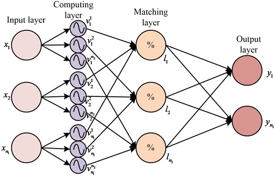
The input of FNN is set as $x_{a} (a = 1,2, \dots, n_{1})$ , and $n_{1}$ is the input quantity. The calculation layer uses Gaussian basis function to calculate the fuzzy membership of each input component, and the function expression is Eq. (10):

10

v_{a}^{b} (x_{a}) = e x p (- {(\frac{x_{a} - c_{a}^{b}}{κ_{a}^{b}})}^{2}), b = 1,2, \dots, n_{2},

where $v_{a}^{b}$ is Gaussian basis function $c_{a}^{b}$ is function center, $κ_{a}^{b}$ is function width in Eq. (10), and their values can be changed. The vectors of its function center and width are $c = {[c_{1}^{1}, \dots c_{1}^{n_{2}}, c_{2}^{1}, \dots c_{n_{1}}^{1}, \dots c_{n_{1}}^{n_{2}}]}^{T} \in R^{N_{f}}$ and $κ = {[κ_{1}^{1}, \dots κ_{1}^{n_{2}}, κ_{2}^{1}, \dots κ_{n_{1}}^{1}, \dots κ_{n_{1}}^{n_{2}}]}^{T} \in R^{N_{f}}$ respectively, where $T$ is transposed and $N_{f} = n_{1} * n_{2}$ . The matching layer is used to match the front row of fuzzy rules, and Eq. (11) is the calculation:

11

l_{b} = \frac{\prod_{a = 1}^{n_{1}} e x p (- {(\frac{x_{a} - c_{a}^{b}}{κ_{a}^{b}})}^{2})}{\sum_{b = 1}^{n_{2}} [\prod_{a = 1}^{n_{1}} e x p (- {(\frac{x_{a} - c_{a}^{b}}{κ_{a}^{b}})}^{2})]},

where $l_{b}$ is fuzzy-regulation. The output layer is clear calculation, and its expression is Eq. (12):

12

y_{o} = \sum_{b = 1}^{n_{2}} w_{a}^{b} l_{b},

where $y_{o} (o = 1,2, \dots n_{3})$ is the output value of FNN, and $w_{a}^{b}$ is the weight coefficient in Eq. (12). The output of FNN can be written in matrix form, and its expression is Eq. (13):

13

y = {[y_{1}, y_{2}, \dots, y_{n_{3}}]}^{T} = W L,

where $y \in R^{n_{3}}$ represents the output vector, $W$ represents the weight coefficient matrix, and $L = {[l_{1}, \dots, l_{n_{2}}]}^{T} \in R^{n_{2}}$ represents the output base vector in Eq. (13). The expression of $W$ is shown in the Eq. (14):

14

W = [\begin{array}{l} w_{1}^{1} & \dots & w_{1}^{n_{2}} \\ ⋮ & ⋱ & ⋮ \\ w_{n_{3}}^{1} & \dots & w_{n_{3}}^{n_{2}} \end{array}] \in R^{n_{3} * n_{2}},

where, $w_{1}^{1}$ is the weight coefficient in the matrix. When designing the controller, the joint angle $p$ and joint angular velocity $\dot{p}$ of the manipulator are set to be measurable, the expected angle $p_{d}$ and its derivative ${\dot{p}}_{d}$ are known, and other parameters are unknown. The expected AFNNC control target is that $p \to p_{d}$ , $\dot{p} \to {\dot{p}}_{d}$ are guaranteed when $t \to \infty$ . The expression of angular error $e$ and angular velocity error $\dot{e}$ is defined in Eq. (15):

15

\{\begin{array}{l} e = p - p_{d}, \\ \dot{e} = \dot{p} - {\dot{p}}_{d} . \end{array}

The sliding surface $s$ is defined as $s = \dot{e} - α e$ . $α$ is an adjustable constant, and $α > 0$ . In Eq. (16), intermediate variable ${\dot{p}}_{r}$ and its derivative ${\ddot{p}}_{r}$ are defined:

16

\{\begin{array}{l} {\dot{p}}_{r} = {\dot{p}}_{d} - α e, \\ {\ddot{p}}_{r} = {\ddot{p}}_{d} - α \dot{e} . \end{array}

Eq. (15) and (16) are substituted into the mechanical arm dynamics in model Eq. (9). And Eq. (17) can be obtained:

17

τ = M \dot{s} + M {\ddot{p}}_{r} + C s + C {\dot{p}}_{r} + G + f + d .

In system friction link, $F$ is approximated by FNN. $F$ is nonlinear function and its expression is Eq. (18):

18

F = W^{*}, c^{*}, κ^{*},

where $W^{*}$ is FNN's ideal weight matrix in Eq. (17). $L^{*} = L (c^{*}, κ^{*}, s)$ is FNN's output vector. The approximation error vector is $ε$ . If the exact value of $W^{*}$ , $c^{*}$ , $κ^{*}$ are unknown and their estimated values are $\hat{W}$ , $\hat{c}$ , $\hat{κ}$ , the approximation error function is changed to Eq. (19):

19

\tilde{F} = W^{*} L^{*} - \hat{W} \hat{L} + ε,

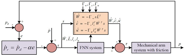
where $\tilde{F}$ is approximate error function, $\hat{W} \hat{L}$ is the actual output of FNN in Eq. (18). The system’s nonlinear factors can be offset to improve controller ability to make unknown nonlinear problems solved. The parameter adaptive law can suppress the influence of approximation error and unknown disturbance of FNN, and Eq. (20) is chosen:

20

\{\begin{array}{l} \dot{\hat{W}} = - Γ_{w} s {\hat{L}}^{T}, \\ \dot{\hat{c}} = - Γ_{c} l_{c}^{T} {\hat{W}}^{T} s, \\ \dot{\hat{κ}} = - Γ_{κ} l_{κ}^{T} {\hat{W}}^{T} s, \end{array}

where $Γ_{w}$ , $Γ_{c}$ , $Γ_{κ}$ are well-dimensioned positive definite diagonal matrices. The AFNNC structure built in the study is shown in Fig. 3.

Fig. 3FNN model of 4-layer structure

3. Analysis of experimental results of manipulator trajectory planning and control methods

3.1. Experimental test of manipulator trajectory planning

To illustrate the effectiveness of JS trajectory planning method based on quintic non-uniform B-spline interpolation, experiments were carried out using MATLAB software. The detailed application scenario is as follows: Kinect V2 camera, Cinder 1920×1080 (32 bits) and 512×424 (16 bits), open frameworks development framework library, Nvidia Jetson Tegra X2 embedded development board master computer (four core ARM A57 Processor, storage size 32GB).The initial joint coordinate is set as $p_{0} = [0 0 0 0 0 0]$ , and the coordinate of the end is mapped as $p_{1} = [40, - 4,40.1]$ through the jocb function in the software. This is the rectangular vertex, and the coordinates of other vertices are $p_{2} = [40,25,40.1]$ , $p_{3} = [10,25,40.1]$ , and $p_{4} = [10, - 4,40.1]$ . When the equidistant value of the rectangular frame is known, the end motion trajectory of the manipulator is planned with cubic polynomial, quintic polynomial and quintic non-uniform B-spline interpolation (5-B interpolation). The angular velocity and angular acceleration curves of each joint are obtained by derivative. Fig. 4 shows the displacement, angular velocity and angular acceleration curves of joint 1 in the range of $t = [2,3]$ .

Fig. 4Joint 1 motion curve of three planning methods

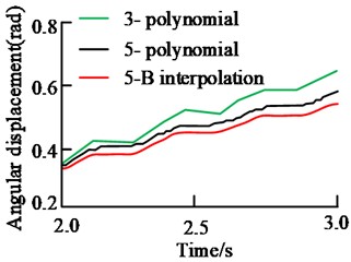
a) Angular displacement curve

b) Angular velocity curve

c) Angular acceleration curve

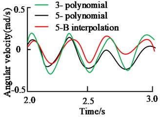
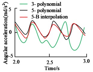
From the angular displacement in Fig. 4 (a), three curves are continuous. When the cubic polynomial is used for trajectory planning, the angular displacement change of joint 1 is 0.26 rad. The change of joint angular displacement in quintic polynomial trajectory planning is 0.24 rad. The angular displacement variation of 5-B interpolation trajectory planning is 0.22 rad. From the change amount and curve smoothness, the curve obtained by 5-B interpolation method is smoother and the number of mutation points is the least. From the angular velocity curve in Fig. 4(b), the curve of cubic polynomial has the largest movement amplitude and moves within ± 0.3 rad/s. The curve inflection point is sharp and the curve smoothness is poor. The change trend of the speed curve of quintic polynomial and 5-B interpolation method is similar. However, the motion trajectory of 5-B interpolation method is smoother, the motion amplitude is smaller, and it moves within ± 0.2 rad/s. The angular acceleration curve of the cubic polynomial in Fig. 4(c) is relatively smooth, but the movement trend is quite different. Compared with the curve of 5-B interpolation method, the trend of quintic polynomial is the same, but the smoothness of 5-B interpolation method is higher.

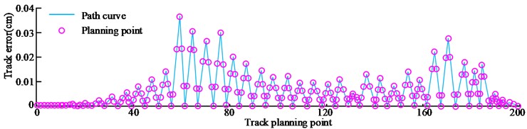
The displacement data of joint 1 is collected at equal time intervals on the planned trajectory, and a total of 200 groups of data are collected. The spatial coordinates corresponding to the displacement data are obtained through the function. The error curve results of the three planned trajectory curves are shown in Fig. 5.

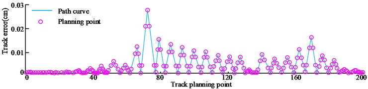
Through the comparison between Fig. 5, the trajectory error of cubic polynomial programming is the highest, and its maximum error value is 0.037 cm. While it is 0.028 cm in the trajectory error of quintic polynomial programming. The trajectory error of the research method planning is the smallest, and its maximum value is 0.026 cm. In the polynomial programming method, the higher the degree, the smaller the planning path error. Quintic polynomial combined with non-uniform B-spline interpolation can improve motion stability and further reduce trajectory error. Table 1 shows the calculation results of trajectory position planning error and velocity error of all joints.

From Table 1, the maximum absolute value of the average position error of each joint is 0.20 rad, and the maximum absolute value of the average speed error is 0.23 rad/s. The average error of the research method is the smallest, the position error is not more than 0.10 rad, and the maximum speed error is 0.09 rad/s. The proposed planning method can better plan the complex motion of the manipulator, and the planning accuracy is higher. It is a stable and reliable trajectory planning method.

Fig. 5Error curves of three kinds of planning trajectory curves

a) 3- polynomial

b) 5- polynomial

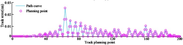
c) 5-B interpolation

Table 1Track planning error result

	Planning method	Joint 1	Joint 2	Joint 3	Joint 4	Joint 5	Joint 6
Mean value of position error (rad)	3-polynomial	–0.18	0.13	–0.19	0.15	–0.20	0.16
	5-polynomial	–0.07	0.08	–0.13	0.09	–0.14	0.08
	5-B interpolation	–0.04	0.05	–0.08	0.04	–0.09	0.06
Mean value of speed error (rad/s)	3-polynomial	–0.23	–0.11	0.22	–0.14	0.17	0.18
	5-polynomial	–0.14	–0.05	0.15	–0.07	0.09	0.11
	5-B interpolation	–0.08	–0.02	0.09	–0.03	0.05	0.07

3.2. Performance impact analysis of trajectory controller under different parameters

For the designed AFNNC, there are many parameters. Different parameters have different effects on the performance of trajectory controller. Firstly, initial values and adaptive rate parameters of different weight coefficient matrices $\hat{W}$ , $\hat{c}$ , $\hat{κ}$ in FNNN are selected to analyze their effects on controller performance. Then, three different Gaussian-based initial values $Γ_{w}$ , $Γ_{c}$ , $Γ_{κ}$ are selected to analyze the trajectory tracking error of the manipulator. The parameters are set as shown in Table 2.

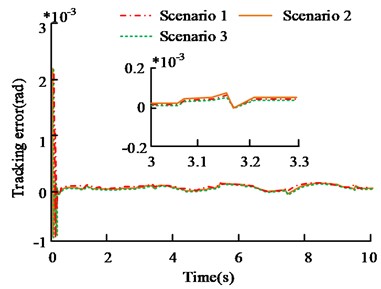
Fig. 6 is the results of manipulator's trajectory tracking error. From Fig. 6, the tracking error results obtained by selecting different FNN weight coefficient matrices are not different. In the 3-3.3 s intercepted in Fig. 6(a), the average tracking error in case 1 is 0.2×10^-5 rad, the average tracking error in case 2 is 0.3×10^-5 rad, and the average tracking error in case 3 is 0.2×10^-5 rad. From the data points, different values have little effect on the tracking error of joint 1. Similarly, from the 5-5.3 s in Fig. 6(b), the average tracking error in case 1 is 0.15×10^-5 rad, the average tracking error in case 2 is 0.25×10^-5 rad, and the average tracking error in case 3 is 0.2×10^-5 rad. It shows that the weight coefficient matrix $\hat{W} (0)$ does not affect the controller performance obviously. This is related to the ability of $\hat{W} (0)$ to update in real time, as long as the initial value of $\hat{W}$ is not too large.

Table 2Parameter settings

Parameter Name	Parameter expression	Parameter setting 1	Parameter setting 2	Parameter setting 3
The initial value of the weight coefficient matrix	$\hat{W}$	D: All elements are 0	E: All elements are 10	F: Random number with all elements ranging from 0 to 10
Adaptive rate parameter	$Γ_{w}$	$Γ_{w} = 1 \times 1 0^{3} I$	$Γ_{w} = 5 \times 1 0^{3} I$	$Γ_{w} = 2 \times 1 0^{4} I$
	$Γ_{c}$	$Γ_{c} = Γ_{κ} = 200$	$Γ_{c} = Γ_{κ} = 50$	$Γ_{c} = Γ_{κ} = 10$
	$Γ_{c}$	$Γ_{c} = Γ_{κ} = 200$	$Γ_{c} = Γ_{κ} = 50$	$Γ_{c} = Γ_{κ} = 10$
The initial value of the Gaussian base function parameter	$\hat{c}$	$c_{a}^{b} (0) = 2 b - 8$	$c_{a}^{b} (0) = b - 4$	$c_{a}^{b} (0) = 0.5 b - 2$
The initial value of the Gaussian base function parameter	$\hat{κ}$	$\hat{κ}$	$κ_{a}^{b} (0) = 1$	$κ_{a}^{b} (0) = 0.5$
Note: $I$ is a good size identity matrix

Fig. 6Track tracking error results of different FNN weight matrices

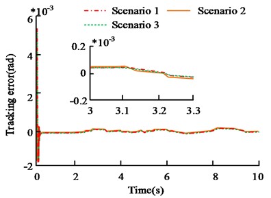
a) Joint 1 tracking error

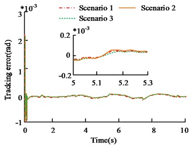
b) Joint 2 tracking error

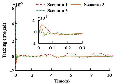
Three different initial values of Gausky are selected for simulation experiments, namely $c_{a}^{b} (0) = 2 b - 8$ , $κ_{a}^{b} (0) = 2$ , $c_{a}^{b} (0) = b - 4$ , $κ_{a}^{b} (0) = 1$ and $c_{a}^{b} (0) = 0.5 b - 2$ , $κ_{a}^{b} (0) = 0.5$ . The results of the trajectory tracking error of the manipulator are shown in Fig. 7. From Fig. 7(a), the tracking error results of different initial values of Gausky function are not significantly different, and the overall trend is basically the same. In Fig. 7(a), from the tracking error results within 5-5.3 s, the average tracking error is 0.2×10^-5 rad, 0.25×10^-5 rad and 0.2×10^-5 rad in case 1~3. In Fig. 7(b), from the tracking error results within 3-3.3 s, the error results of the three cases are 0.25×10^-5 rad, 0.33×10^-5 rad and 0.3×10^-5 rad respectively. The tracking error of the three cases is less than 0.1×10^-5 rad. The selection of Gaussian basis function's initial value affects controller performance slightly, and there is no obvious difference between different values. Therefore, the parameter selection in the process of building the controller using FNN is relatively simple. According to tracking system's response, it can adjust FNN's parameters in real time.

In the controller, for the adaptive parameters $Γ_{w}$ , $Γ_{c}$ , $Γ_{κ}$ , different $Γ_{w}$ is first selected for experiments. Then different parameters $Γ_{c}$ , $Γ_{κ}$ of Gausky adaptive law are set for the experiment. The tracking error results obtained by different adaptive law parameters are shown in Fig. 8.

Fig. 8(a) shows the track tracking error results under different $Γ_{w}$ values. The selection of $Γ_{w}$ and the convergence rate of tracking error as well as steady-state error have an impact. When the value of $Γ_{w}$ is small, the error convergence speed is slow, about 0.14 s before convergence. And the fluctuation range of steady-state error is large, within ±0.1×10^-3 rad. It is possible that $Γ_{w}$ is too small, so FNN's performance is restricted to approach performance of nonlinear links, resulting in poor tracking performance of the controller. When $Γ_{w}$ is large, its convergence speed is faster. It completes convergence in about 0.07 s, and has small steady-state error. However, when $Γ_{w}$ is too large, the steady-state error fluctuates, with a range of ±0.3×10^-4 rad. It shows that different $Γ_{w}$ values will affect controller tracking performance, and this value should not be too large. Fig. 8(b) shows the tracking error results of different B values. The value of $Γ_{c}$ , $Γ_{κ}$ is too small (case 3), and the tracking error is relatively large. Within 1-2 s, the maximum error is 0.9×10^-4 rad, and the error difference of other values is not large. It shows that the value of $Γ_{c}$ , $Γ_{κ}$ cannot be too small, and the appropriate size can improve the robustness of the controller.

Fig. 7Track tracking error results of different initial values of FNN Gaussian basis function

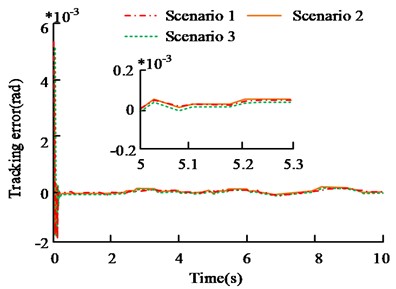
a) Joint 1 tracking error

b) Joint 2 tracking error

Fig. 8Tracking error results of different adaptive law parameters

a) Tracking error of different $Γ_{w}$

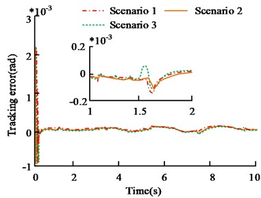
b) Tracking error of different $Γ_{c}$ , $Γ_{κ}$

According to Fig. 6-8, parameters $\hat{W}$ , $\hat{c}$ , $\hat{κ}$ of FNN have little influence on the controller, and they are selected only by experience. For the adaptive law parameters $Γ_{w}$ , $Γ_{c}$ , $Γ_{κ}$ , the selection has relation with the FNN nonlinear function approximation performance, and the larger value is required. $Γ_{c}$ , $Γ_{κ}$ mainly affect the robustness of sudden disturbance of the system, taking the appropriate value. Therefore, the initial value of the weight coefficient matrix is taken as its value of 10.

3.3. Performance test and analysis of manipulator trajectory controller

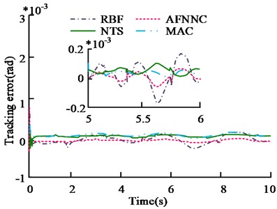
In order to illustrate and study the trajectory tracking performance of the AFNNC controller, the radial basis function (RBF) auxiliary controller was selected for comparison with the space robot motion trajectory planning method based on non-singular terminal sliding mode control (NTS) in reference [5] and the multi-avoidance constraint (MAC) dual-arm space robot coordination trajectory planning method in reference [6]. All control strategies adopt the strategy that nonlinear function compensation with sliding mode control. The friction coefficient of the robot joint is changed from 0.75 to 1.0. When the friction coefficient changes abruptly, the tracking error results of the two controllers are shown in Fig. 9.

Fig. 9Tracking error result of abrupt change of friction coefficient

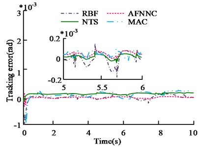
a) Joint 1

b) Joint 2

From Fig. 9(a), for joint 1, when the friction coefficient changes abruptly, the convergence speed of AFNNC is faster than that of RBF controller. Its track tracking error mainly fluctuates in the range of ±0.2×10^-5 rad. The error fluctuation range of RBF is ±0.2×10^-4 rad. NTS and MAC have a wider error range. For joint 2, the track tracking error of AFNNC fluctuates within ±0.2×10^-5 rad, and the error of RBF fluctuates within ±0.3×10^-4 rad. The error ranges for NTS and MAC are ±0.4×10^-4 rad and ±0.35×10^-4 rad. It shows that the performance of AFNNC controller studied is better.

When the load suddenly changes from 2 kg to 3 kg, RBF and FNN are used in the experiment to compare the approximation error of the nonlinear function. Fig. 10 shows the results.

From Fig. 10(a), when the load suddenly changes ( $t =$ 5 s, $t =$ 17 s), the functions will jump. The approximate function curve of FNN has the same trend as the original function, and the fitting effect is better. In Fig. 10(b), the approximation error curve of FNN converges faster and has less response time in case of sudden change. The response time is within 0.03 s and the error range is ±2 Nm. This is because the two control strategies are used to approximate the nonlinear function, so the control effect is directly influenced by nonlinear function. The other two strategies show no such characteristics. Table 3 shows the error comparison results of the 4 controllers when the load changing sudden.

From Table 3, the jump error of AFNNC is 2×10^-4 rad when $t =$ 5 s, and 0.6×10^-3 rad when $t =$ 17 s, which is lower than RBF. Its steady-state error is 0.5×10^-4 rad, and the error is 1×10^-4 rad lower, indicating that AFNNC has better tracking accuracy. The jump error and steady-state error of NTS and MAC are much larger than that of AFNNC. When the AFNNC control strategy is adopted, better accuracy and robustness occurs.

Fig. 10Error results of nonlinear function approximation

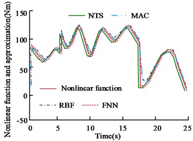
a) Nonlinear function and approximation

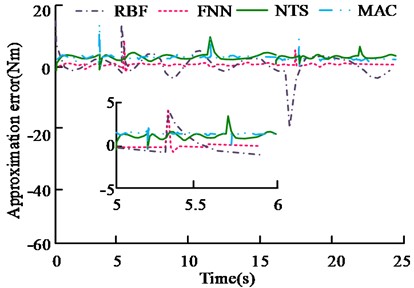
b) Approximation error of nonlinear function

Table 3Error results of 4 controllers at the time of sudden load change

Controller	$t =$ 5 s Jump error	$t =$ 17 s Jump error	Steady-state error
RBF	7×10^-4rad	1.1×10^-3rad	1.5×10^-4rad
AFNNC	2×10^-4rad	0.6×10^-3rad	0.5×10^-4rad
NTS	8×10^-4rad	1.5×10^-3rad	1.42×10^-4rad
MAC	6×10^-4rad	1.3×10^-3rad	1.26×10^-4rad

4. Conclusions

With the expansion of the manufacturing industry, the operation task of the manipulator becomes more and more complex. This also brings challenges to the manipulator. The existing methods have large planning error and poor tracking accuracy. So the planning method of quintic non-uniform B-spline interpolation is proposed, and a trajectory tracking controller based on FNN is designed. The experimental results are as follows:

1) The experimental results of trajectory planning show that the curve of 5-B interpolation trajectory planning is smoother, and the motion amplitude fluctuates within ±0.2 rad/s. The error of 5-B interpolation trajectory planning is the smallest, and its maximum value is 0.026 cm.

2) The results of position planning error and velocity error show that the average error of the research method is the smallest, and the position error does not exceed 0.10 rad, and the maximum velocity error is 0.09 rad/s. The proposed 5-B interpolation planning method can better plan the complex motion of the manipulator, and the planning accuracy is higher.

3) Through the controller tracking experiments under different parameter values, it is found that $\hat{W}$ , $\hat{c}$ , $\hat{κ}$ have little influence on the controller, and the adaptive law parameters have a great influence.

4) Through the AFNNC tracking experiment, the results show that its track tracking error mainly fluctuates in the range of ±0.2×10^-5 rad. In case of sudden load change, the response time of FNN is shorter, and the error range of function approximation is ±2 Nm. When the AFNNC control strategy is adopted, it shows higher accuracy and robustness.

Although the research has achieved certain results, there are still many deficiencies. The simulation platform mainly uses MATLAB software to analyze, and fails to consider the impact of complex actual environment on the manipulator. In the future, more convincing experimental results will be obtained in combination with the actual working environment.

References

Y. Du and Y. Chen, “Time optimal trajectory planning algorithm for robotic manipulator based on locally chaotic particle swarm optimization,” Chinese Journal of Electronics, Vol. 31, No. 5, pp. 906–914, Sep. 2022, https://doi.org/10.1049/cje.2021.00.373

Publisher
Q. Xie, Q. Meng, Q. Zeng, H. Yu, and Z. Shen, “An innovative equivalent kinematic model of the human upper limb to improve the trajectory planning of exoskeleton rehabilitation robots,” Mechanical Sciences, Vol. 12, No. 1, pp. 661–675, Jun. 2021, https://doi.org/10.5194/ms-12-661-2021

Publisher
H. Chang, S. Wang, and P. Sun, “Dynamic output feedback control for a walking assistance training robot to handle shifts in the center of gravity and time-varying arm of force in omniwheel,” International Journal of Advanced Robotic Systems, Vol. 17, No. 1, p. 172988141984673, Jan. 2020, https://doi.org/10.1177/1729881419846737

Publisher
N. Lotti et al., “Myoelectric or force control? A comparative study on a soft arm exosuit,” IEEE Transactions on Robotics, Vol. 38, No. 3, pp. 1363–1379, Jun. 2022, https://doi.org/10.1109/tro.2021.3137748

Publisher
W. Yan, Y. Liu, Q. Lan, T. Zhang, and H. Tu, “Trajectory planning and low-chattering fixed-time nonsingular terminal sliding mode control for a dual-arm free-floating space robot,” Robotica, Vol. 40, No. 3, pp. 625–645, Mar. 2022, https://doi.org/10.1017/s0263574721000734

Publisher
S. Ni, W. Chen, H. Ju, and T. Chen, “Coordinated trajectory planning of a dual-arm space robot with multiple avoidance constraints,” Acta Astronautica, Vol. 195, pp. 379–391, Jun. 2022, https://doi.org/10.1016/j.actaastro.2022.03.024

Publisher
D. Kaljaca, B. Vroegindeweij, and E. Henten, “Coverage trajectory planning for a bush trimming robot arm,” Journal of Field Robotics, Vol. 37, No. 2, pp. 283–308, Mar. 2020, https://doi.org/10.1002/rob.21917

Publisher
X. Yu, M. Dong, and W. Yin, “Time-optimal trajectory planning of manipulator with simultaneously searching the optimal path,” Computer Communications, Vol. 181, No. 1, pp. 446–453, Jan. 2022, https://doi.org/10.1016/j.comcom.2021.10.005

Publisher
Q. Hu, D. Zhang, and Z. Wu, “Trajectory planning and tracking control for 6‐DOF Stanford manipulator based on adaptive sliding mode multi‐stage switching control,” International Journal of Robust and Nonlinear Control, Vol. 31, No. 14, pp. 6602–6625, Sep. 2021, https://doi.org/10.1002/rnc.5628

Publisher
Y. Zhang, M. Li, and C. Yang, “Robot learning system based on dynamic movement primitives and neural network,” Neurocomputing, Vol. 451, pp. 205–214, Sep. 2021, https://doi.org/10.1016/j.neucom.2021.04.034

Publisher
Y. Uno, T. Suzuki, and T. Kagawa, “Repetitive control for multi-joint arm movements based on virtual trajectories,” Neural Computation, Vol. 32, No. 11, pp. 2212–2236, Nov. 2020, https://doi.org/10.1162/neco_a_01322

Publisher
X. Tian and Y. Xu, “Low delay control algorithm of robot arm for minimally invasive medical surgery,” IEEE Access, Vol. 8, pp. 93548–93560, 2020, https://doi.org/10.1109/access.2020.2995172

Publisher
J. Xia, Z.-N. Jiang, and T. Zhang, “Feasible arm configurations and its application for human-like motion control of s-r-s-redundant manipulators with multiple constraints,” Robotica, Vol. 39, No. 9, pp. 1617–1633, Sep. 2021, https://doi.org/10.1017/s0263574720001393

Publisher
G. Wu, W. Zhao, and X. Zhang, “Optimum time-energy-jerk trajectory planning for serial robotic manipulators by reparameterized quintic NURBS curves,” Proceedings of the Institution of Mechanical Engineers, Part C: Journal of Mechanical Engineering Science, Vol. 235, No. 19, pp. 4382–4393, Oct. 2021, https://doi.org/10.1177/0954406220969734

Publisher
Z. Hu, H. Yuan, W. Xu, T. Yang, and B. Liang, “Equivalent kinematics and pose-configuration planning of segmented hyper-redundant space manipulators,” Acta Astronautica, Vol. 185, No. 3, pp. 102–116, Aug. 2021, https://doi.org/10.1016/j.actaastro.2021.04.018

Publisher
A. T. Phan, H. N. Thai, C. K. Nguyen, Q. U. Ngo, H. A. Duong, and Q. T. Vo, “Trajectory tracking control design for dual-arm robots using dynamic surface controller,” Engineering Journal, Vol. 24, No. 3, pp. 159–168, May 2020, https://doi.org/10.4186/ej.2020.24.3.159

Publisher
T. Xu, H. Zhou, S. Tan, Z. Li, X. Ju, and Y. Peng, “Mechanical arm obstacle avoidance path planning based on improved artificial potential field method,” Industrial Robot: the International Journal of Robotics Research and Application, Vol. 49, No. 2, pp. 271–279, Feb. 2022, https://doi.org/10.1108/ir-06-2021-0120

Publisher

About this article

Received

14 March 2023

Accepted

28 June 2023

Published

08 August 2023

SUBJECTS

Vibration control, generation and harvesting

DOI

https://doi.org/10.21595/jve.2023.23274

Keywords

robot

mechanical arm

track planning

FNN

controller

Acknowledgements

The authors have not disclosed any funding.

Data Availability

The datasets generated during and/or analyzed during the current study are available from the corresponding author on reasonable request.

Conflict of interest

The authors declare that they have no conflict of interest.

This is an open access article distributed under the Creative Commons Attribution License, which permits unrestricted use, distribution, and reproduction in any medium, provided the original work is properly cited.

Previous article in issue Previous Next article in issue Next

Research article

2023 01 30

Dynamic obstacle avoidance and trajectory planning of five-axis redundant industrial manipulator

Jian Ma

Research article

2021 08 11

Optimization of trajectory tracking control of 3-DOF translational robot use PSO method based on inverse dynamics control for surgery application

Ngoc Pham Van Bach, Quan Dam Hai, Thanh Bui Trung

Research article

2021 03 26

Trajectory planning for mobile manipulators with vibration reduction

Grzegorz Pajak

Research article

2018 12 31

Dynamic modeling and simulation of three-member robot manipulator

Hristijan Mickoski, Ivan Mickoski, Marjan Djidrov

J. Liu, “Trajectory planning and control algorithm of industrial robot manipulator,” Journal of Vibroengineering, Vol. 25, No. 8, pp. 1516–1530, Aug. 2023, https://doi.org/10.21595/jve.2023.23274

Copy Extrica

Copied to clipboard!

TY  - JOUR
DO  - 10.21595/jve.2023.23274
UR  - https://doi.org/10.21595/jve.2023.23274
TI  - Trajectory planning and control algorithm of industrial robot manipulator
T2  - Journal of Vibroengineering
AU  - Liu, Jing
PY  - 2023
DA  - 2023/08/08
PB  - JVE International Ltd.
SP  - 1516-1530
VL  - 25
IS  - 8
SN  - 1392-8716
SN  - 2538-8460
ER  - 

Copy Ris

Copied to clipboard!

 @article{Liu_2023, title={Trajectory planning and control algorithm of industrial robot manipulator}, volume={25}, ISSN={2538-8460}, url={https://doi.org/10.21595/jve.2023.23274}, DOI={10.21595/jve.2023.23274}, number={8}, journal={Journal of Vibroengineering}, publisher={JVE International Ltd.}, author={Liu, Jing}, year={2023}, month=aug, pages={1516–1530} }

Copy Bibtex

Copied to clipboard!

[1]J. Liu, “Trajectory planning and control algorithm of industrial robot manipulator,” Journal of Vibroengineering, vol. 25, no. 8, pp. 1516–1530, Aug. 2023, doi: 10.21595/jve.2023.23274.

Copy IEEE

Copied to clipboard!

Liu, Jing. “Trajectory Planning and Control Algorithm of Industrial Robot Manipulator.” Journal of Vibroengineering 25, no. 8 (August 8, 2023): 1516–30. https://doi.org/10.21595/jve.2023.23274.

Copy Chicago

Copied to clipboard!

Trajectory planning and control algorithm of industrial robot manipulator

Abstract

1. Introduction

2. Research on trajectory planning and control method of manipulator JS

2.1. JS trajectory planning based on quintic non-uniform B-spline interpolation

2.2. JS trajectory tracking control of manipulator based on FNN

3. Analysis of experimental results of manipulator trajectory planning and control methods

3.1. Experimental test of manipulator trajectory planning

3.2. Performance impact analysis of trajectory controller under different parameters

3.3. Performance test and analysis of manipulator trajectory controller

4. Conclusions

References

About this article

Related Articles