Automatic vibration control method for grasping end of flexible joint robot

3.1. Dynamic model construction of end vibration of FJB

The accurate dynamic model construction of FJB is the basis of achieving high-precision control and vibration suppression. For the analysis of dynamic model of FJB, Newton-Euler method is used for vector mechanics modeling in this study. Newton-Euler modeling is based on Newton’s equation and Euler’s equation. By analyzing the speed and acceleration of each link of the manipulator, the interaction force between each link is determined. At the same time, the experiment completed the derivation of the overall dynamic model of the robot through chain iteration. The Newton-Euler model clarifies the interaction forces between the links, which is more conducive to the design of control algorithms for flexible robots. Due to the complex content and structure of the flexible joint, the robot joint is equivalent to the linear torsion spring proposed by Spong. The equivalent model is shown in Fig. 1.

Fig. 1Equivalent model of robot flexible joint

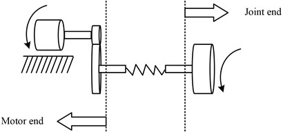
It can be seen from Fig. 1 that the elastic force generated by joint flexibility and joint torsion form become linear. The proportional coefficient is the elastic coefficient of the spring. This model concentrates the mass of the rotor on the shaft. Before building the dynamic model of FJB, to simplify the mechanical structure and calculation process, the subsequent presumptions are first proposed: (1) The flexible joint is equivalent to the Spring model, that is, the linear torsion spring, and the spring force is linear with the joint shape variables. (2) Ignoring the influence of the motor rotor, it is assumed that the motor rotor is coaxial with the joint axis. (3) Without considering the coupling effect of motor dynamics and robot dynamics, it is assumed that the motor is a perfect source of torque and that its reaction time is adequate. (4) It is assumed that the mass of the connecting rod is uniformly distributed and the connecting rod will not deform, and the position of the connecting rod centroid is 1/2 of the length of the connecting rod. Set the ideal torque of motor output as ${\tau }_{motor,i}$; The torque changes to $r_i$ after the transmission of the reducer with a reduction ratio of ${\tau }_{l,i}$. The motor output angle is ${\theta }_{motor,i}$; The actual output angle is ${\theta }_{l,i}$ after decelerating by the reducer. The moment of inertia of the motor rotor is $J_{motor,i}$, and the moment of inertia after deceleration is $J_{l,i}$. The relationship between the three decelerator before and after conversion is expressed as the following Eq. (1):

where, $l$, $i$ all indicate the connecting rod number. When the joint stiffness is insufficient, the robot joint will undergo small deformation. That is, the connecting rod’s angle and the reducer’s output rotation angle are not equivalent., and its relationship is expressed as Eq. (2):

where, $i$ represents the number of flexible joints; ${\tau }_i$ indicates the driving torque of the $i$-th connecting rod; $K_i$ indicates the elastic coefficient of the torsion spring. $q_i$ indicates the actual angle of the $i$ connecting rod. As stated by the Newtonian dynamics formula $F=ma=m\frac{dv}{dt}$ and the description of rotation motion in Euler equation, the dynamic moment generated by rotation is expressed as Eq. (3):

where, ${\rho }_i$ denotes the radius of rotation; $m_i$ indicates the centroid mass; $\omega$ denotes the linear speed of the centroid rotation. $v_i$ is the center of mass's moment of inertia; $I$ represents the rotational angular speed of the centroid. Therefore, according to the theorem of moment of momentum, the resultant moment of the resultant force on the fulcrum is expressed as $M=\frac{dJ}{dt}=J\text{'}+\omega \times I\omega$. According to the recursive algorithm of Newton-Euler method, the extrapolation formula of velocity and acceleration on both banks is expressed as Eq. (4):

where, ${}^{i+1}\mathrm{}{F}_{i+1}^{}$ represents the resultant force on the centroid of connecting rod $i+1$; ${}^{i+1}\mathrm{}{N}_{i+1}^{}$ is expressed as the resultant time on the centroid of the connecting rod $i+1$. ${}^{i+1}\mathrm{}{v\text{'}}_{Ci+1}$ expressed as the acceleration of the centroid of the connecting rod $i+1$; ${}^{Ci+1}\mathrm{}{I}_{i+1}$ represents the inertia tensor of the center of mass of the connecting rod $i+1$; ${\omega }_{i+1}$ and ${\omega \text{'}}_{i+1}$ respectively represent the angular velocity and angular acceleration of the connecting rod $i+1$. The connecting rod's driving power and torque are expressed in Eq. (5):

where, ${}^i\mathrm{}{f}_i$ and ${}^i\mathrm{}{n}_i$ represent the force and moment at joint $i$; ${\tau }_i$ is the driving torque of the joint. ${}_{i+1}{}^i\mathrm{}{R}^{i+1}$represented as the rotation matrix from coordinate system $i$ to coordinate system $i+1$; ${}^{i+1}\mathrm{}{Z}_{i+1}=[\mathrm{0,0},1{]}^T$, ${}^i\mathrm{}{P}_{i+1}$ represents the position of the coordinate system $i+1$ relative to the coordinate system $i$; ${}^i\mathrm{}{P}_{Ci}$ represented as the centroid position of the connecting rod $i$. Finally, improve the friction term and joint inertia in the dynamic model, and Eq. (6) shows it:

where, ${\tau }_F$ represents the friction model; ${\tau }_J$ represents joint inertia force. $f_v$ represents viscous friction, and $f_c$ represents coulomb friction. Finally, the dynamic model of the FJB can be expressed by combining the Eq. (2):

where, $M\left(q\right)$ denotes the robot’s connecting rod’s inertia matrix; $C(q,q\text{'})$ is the centrifugal force matrix; $G\left(q\right)$ indicates the gravity vector; ${\tau }_d$ denotes the uncertain interference term of robot joint; $\tau$ denotes the torque of the connecting rod. To apply the property expression, after building the dynamic model of the FJB, the research will express the dynamic characteristics of the robot through the mathematical model. In the feature of parameter linearization, set the function $n*m$ with $Y(q,q\text{'},q\text{'}\text{'})$ and the dimension vector $m$ of $\mathrm{\Theta }$, so that the robot dynamics formula can be written into Eq. (8):

3.2. Optimization of SMC based on RBF neural network error compensation

The vibration control of conventional FJB adopts PID control, sliding mode variable structure control, singular perturbation method, neural network control, adaptive control, etc. In this research, to improve SMC for vibration suppression, a neural network is utilized. The chattering effect of SMC is often caused by the modeling error of the system and the sign function in the control rate. Therefore, to eliminate the chattering phenomenon, it is required to consider two aspects: compensating the modeling error and changing the control rate structure. In this study, RBF model is used to enhance SMC. RBF neural network universal approximation principle is used to compensate the modeling error of the system online.

Fig. 2RBF neural network optimization process for SMC

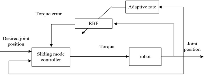
As shown in Fig. 2, in this vibration suppression method, the optimization of SMC mainly uses Lyapunov method to derive the neural network weight adaptive rate. In the experiment, RBF neural network is used for data set training, and the goal of stable convergence of the control system is finally achieved. First, the position error is defined as $e\left(t\right)=q_d\left(t\right)-q\left(t\right)$; The velocity error is $e\text{'}\left(t\right)={q\text{'}}_d\left(t\right)-q\text{'}\left(t\right)$. Therefore, the system modeling error is expressed as Eq. (9) by combining Eq. (8):

where, the system error is related to the actual angle $q$, actual angular velocity $q\text{'}$, actual angular acceleration $q\text{'}\text{'}$, joint angular error $e$, joint angular speed error $e\text{'}$, and joint angular acceleration error $e\text{'}\text{'}$ of the robot joint. Set the above parameters as the input of the neural network, namely $x=[e^T,{e\text{'}}^T,{e\text{'}\text{'}}^T,q^T,{q\text{'}}^T,{q\text{'}\text{'}}^T]$. If the RBF network is applied to compensate the system modeling deviation, the network output under ideal conditions is expressed as Eq. (10):

where, $W$ denotes the network’s ideal weight matrix; $\mathrm{\Phi }\left(x\right)$ is radial basis function’s output; $\mathrm{\Delta }E$ indicates the error of neural network. Assume that RBF’s true output is $\mathrm{\Delta }\widehat{\tau }=W\mathrm{\Phi }\left(x\right)$. Take $\stackrel{-}{W}=W-\widehat{W}$ to represent the deviation between the true weight and the ideal weight; Then the SMC law of the robot can be set as Eq. (11) based on the nominal model ${\tau }_s=\mathrm{\Psi }+\lambda s+\sigma \mathrm{s}\mathrm{g}\mathrm{n}\left(s\right)$:

where, $\mathrm{\Psi }$ represents the nominal model; (A $s\left(t\right)=e\text{'}+\beta e$) is the error description function; $\lambda$ is the weight of convergence rate; $\sigma$ is the weight of robot vibration. $k_{\sigma }$ represents the resilient term coefficient to cancel the system's uncertain disturbance. To derive the weight adaptive rate, the Lyapunov function is defined as: $V=\frac{1}{2}{s}^T(M+J)s+\frac{1}{2}tr\left({\stackrel{-}{W}}^T{\mathrm{\Gamma }}^{-1}\stackrel{-}{W}\right)$. There are:

where, $tr\left(\right)$ represents the trace of the matrix; $\mathrm{\Gamma }$ represents a matrix of symmetric positive definite constants. As stated by the characteristics of the robot dynamics model built in the previous section, it can be concluded that: $x^T\left[M\text{'}\right(q)-2C(q,q\text{'}\left)\right]x=0$, so the Lyapunov function can be modified to Eq. (13):

Substituting neural SMC law Eq. (11) into Eq. (13), the following Eq. (14) can be obtained:

It can be seen from the circular nature of the matrix trace that when there is a symmetric relationship between different matrices of the same dimension, the trace of their scores will not change under all the rings; At the same time, when the product of all cyclic sequences still exists, their traces will still be identical, but only satisfy the product of cyclic positions, not the product of all $p$:

To make the derivative of Lyapunov function less than 0, take $\left\{\begin{array}{l}{k}_{\sigma }>‖\mathrm{\Delta }E‖+‖{\tau }_d‖\\ \stackrel{-}{W\text{'}}=-\mathrm{\Gamma }\mathrm{\Phi }\left(x\right)s^T\end{array}\right.$. Once the neural network design is completed, $‖\mathrm{\Delta }E‖$ will approach 0. Therefore, the value of $k_{\sigma }$ will be far less than the sliding and grinding switching coefficient in the traditional SMC law, thus achieving the effect of weakening the robot vibration. At the same time, the expected weight $\stackrel{-}{W}=W-\widehat{W}$ in $W$ is regarded as a constant. Therefore, the adaptive rate is expressed as Eq. (16):

4.1. Simulation experiment of two-joint flexible robot under SMC

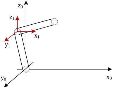
To test the control performance of the SMC strategy, experiments and practical application analysis are carried out on the two-joint flexible robot and the six-joint flexible robot respectively. First, in the experiment of two-joint flexible robot, set the control proportion parameter as [3000 2900] T; The coefficient of differential link is [250 120] T. Set the position error weight parameter as [20 2.34] T; The weight parameter of convergence speed is [2017] T; The robot vibration weight parameter is [10 120] T. The simulation model is built through simulink in this experiment. The model of the experimental object of the two-joint robot is shown in Fig. 3.

Fig. 3Dynamic model of 2-joint flexible robot

After building the simulation model through Simulink, this study first compares the feedforward PD control with the SMC model in this paper. First, a non-interference simulation experiment is carried out. The position tracking curve of robot joint 1 by two control methods is as shown in Fig. 4.

Fig. 4Position curve and error curve of joint 1 of two-joint robot under different control methods

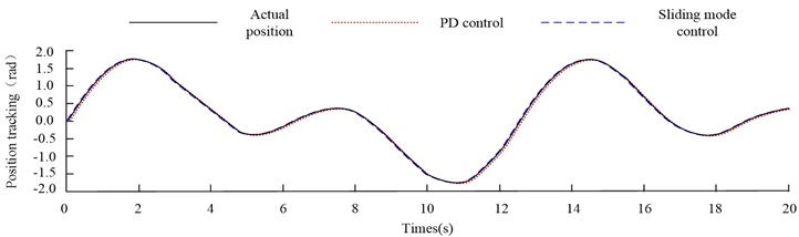
a) Position tracking

b) Position tracking error

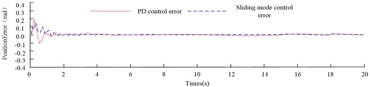
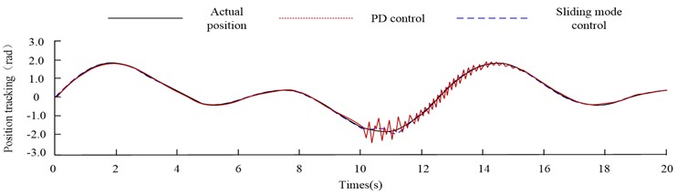
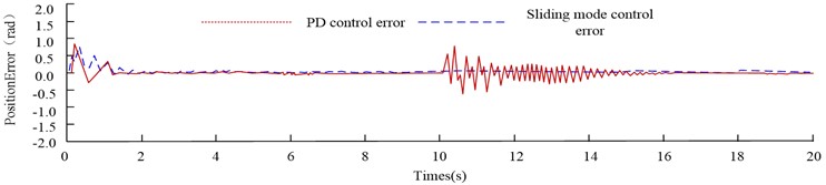
From Fig. 4(a), under the two control methods, the two-joint flexible robot achieves stable tracking of the desired position curve after 1.5 s. From Fig. 4(b), when the feedforward PD control mode is adopted, the first joint's maximum inaccuracy is around 0.17 rad.; The maximum error of the first joint under the SMC method is about 0.15 rad. In order to comprehensively evaluate the performance of the control method, the average absolute error (MAE) is used to describe the average error in the experiment. After calculation, the MAE of PD control is 0.02111 rad. The MAE of SMC is 0.0151 rad. From the data, both control methods can reach stable control of the two-joint robot in the non-interference environment. However, the control effect of SMC is better than that of feedforward PD control. In order to analyze the anti-jamming ability of different control methods, this experiment will apply a pulse signal with amplitude of 0.5 rad to the robot's position feedback when the system runs for 10 s, so as to simulate the uncertain interference when the robot runs. Therefore, the control of joint 1 by different control methods in the interference environment is shown in Fig. 5.

Fig. 5Control of joint 1 by different control methods under interference environment

a) Position tracking

b) Position tracking error

From Fig. 5(a), the two control methods have different degrees of error after the pulse interference is applied. The maximum error of the feedforward PD control method reaches 1 rad and the recovery time reaches 5 s. The maximum deviation of the SMC method is only about 0.25 rad; the recovery time is only about 1 s. Therefore, the SMC method has stronger robustness and higher ability to resist uncertain disturbances. Finally, the experimental data of the two joints of the flexible robot are shown in Table 1.

From Table 1, SMC is better than feedforward PD control in terms of maximum system error and average absolute error, and SMC has stronger anti-interference ability. When pulse interference is applied, the recovery time is faster and the error caused is smaller.

4.2. Experimental analysis of 6-joint flexible robot under SMC with RBF neural network error compensation

This experiment uses Simscape Multibody to build a 6-DOF cooperative manipulator with flexible joints. In Simscape, the robot dynamics model can be quickly built. In addition, the experiment can simulate the torque sensor, encoder and other components to obtain relevant data. The link mass, gravity acceleration and other information can be defined in the solid model. Simscape can be displayed in the form of simulink module, and then generate animation to observe the operation of the robot. Fig. 6 illustrates the generated robot model.

Fig. 66-DOF robot model with flexible joints

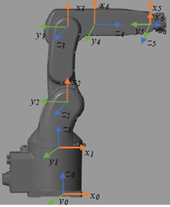
As shown in Fig. 6, the 6-joint robot of the experimental object is designed with reference to the human arm joint, which is divided into waist joint (the first joint), shoulder joint (the second joint), elbow joint (the third joint), wrist joint 1 (the fourth joint), wrist joint 2 (the fifth joint) and wrist joint 3 (the sixth joint). Referring to the dynamic model in the study, Table 2 demonstrates the dynamic parameters of the robot.

In addition to the dynamic parameters of the robot in Table 2, RBF combined with SMC is adopted in this study. The control rate parameters are [3.5×107, 3.5×107, 2.2×107, 3×106, 1.5×106, 1.7×106] T; The sliding surface parameter is [400382300130, 20, 12] T; The sign function coefficient is [70000100000011000040001000800] T. The radial base width of neurons is 100; The adaptive rate parameter is diag (5, 5, 15, 5, 10, 5). To test the tracking effect of SMC algorithm on different trajectories, 11 path points are selected in Cartesian space to make the end of the manipulator move along the path points. After RBF-sliding mode control planning and PD control planning, the velocity and acceleration of the robot end are shown in Fig. 7.

Fig. 7Velocity and acceleration of robot end under two control methods

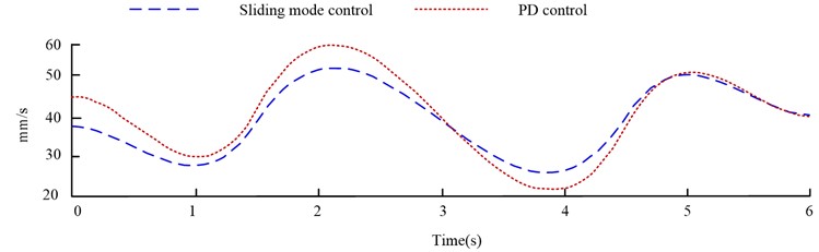
a) The speed of robot controlled by different methods

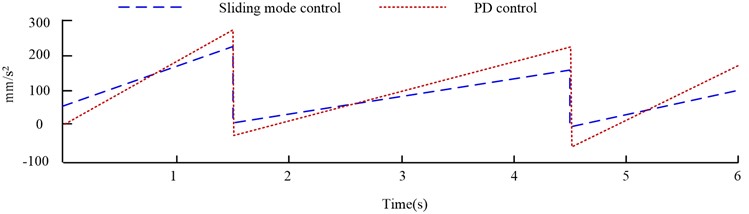
b) Acceleration of robot controlled by different methods

From Fig. 7(a), the end velocity of the 6-joint robot is between 30 mm/s and 50 mm/s through RBF-sliding mode control planning; The terminal speed controlled by PD is between 20 mm/s and 60 mm/s. The data shows that the end speed of the robot controlled by RBF - sliding mode is more stable. As can be seen from Fig. 7 (b), when the control rate is switched at a high frequency, both control techniques cause the robot to chatter. PD control robot has discontinuous and non-smooth phenomenon, and also has more obvious jump. The occurrence of this situation will cause a heavy burden on the controller and easily lead to the phenomenon of control instability. At the same time, it will also aggravate the wear of the mechanical arm and other problems. However, the method proposed in the study has a light jump phenomenon and has a better effect on the vibration control of the robot end. From Fig. 8, This research simulates the Cartesian space trajectory of the robot end under the control of the two techniques, as well as observes and analyzes the robot end’s trajectory tracking control effect under the two control methods.

Fig. 8Cartesian space robot trajectory tracking diagram

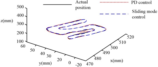
From Fig. 8, the two models have better tracking effect on the part of straight line track, and slightly worse tracking effect on the arc track. The reason is that the arc trajectory needs the robot’s centripetal force at each joint to make the robot end complete the arc motion. However, due to the existence of joint flexibility, it is difficult to provide enough centripetal force, which leads to tracking error. From the card in Fig. 8, the maximum tracking error of the traditional PD control exceeds 5 mm, while the maximum error of the optimized Sliding mode control method is within 3 mm. On the whole, the effect of the improved neural network SMC algorithm is better than PD control algorithm. The robustness of SMC overcomes the tracking error caused by joint flexibility to a certain extent. Finally, the three-axis error of the two robot control methods under the trajectory tracking experiment is compared, as shown in Fig. 9.

Fig. 9Three-axis error comparison of different control methods on the end track

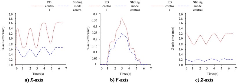
From Fig. 9, there are some flaws in the flexible manipulator’s movements in all three directions, and the error of the robot under PD control in the three directions is higher than that of the SMC-RBF method. In Fig. 9(a), the robot’s maximum error end on the $X$-axis under PD control is 1.6 mm; The maximum error of the robot under RBF-sliding mode control is only 0.7 mm; The maximum error of the neural network optimization method on the $X$ axis is 0.9 mm less than that of the traditional method. From Fig. 9(b), the maximum error of the neural network optimization method on the $X$-axis is 0.1mm less than that of the traditional method. The biggest error is 0.25 mm; The biggest error of traditional PD control is 0.35 mm. From Fig. 9(c), the biggest error of the method in this study on the $z$-axis is 1.25 mm; The biggest error of the robot under PD control method is 2.2 mm; After optimization, the maximum error of $z$-axis is reduced by 0.95 mm. Finally, this study uses MAE to comprehensively describe the control error in each direction under the two controls, as shown in Table 3.

From Table 3, the average absolute error of the SMC-RBF in this study on the three axes is 0.505 mm, 0.092 mm and 1.158 mm respectively; The traditional PD control method’s average absolute error on the three axes is 1.219 mm, 0.254 mm and 1.995 mm respectively. It is obviously that the control method that optimizes the SMC method through RBF can effectively weaken the end vibration of the robot.