Abstract
When tracking the trajectory of the mechanical arm in a joint space, the system is affected by friction non-linearity, unknown dynamic parameters and external disturbances that makes it difficult to improve the control accuracy of the mechanical arm. To solve the above problems, this paper introduces LuGre friction model and designs a new joint space trajectory tracking controller based on the adaptive fuzzy neural network. The controller is capable to make the adaptive adjustment of the center and width of the basis function, can approach the nonlinear link having the LuGre friction on line, and uses the sliding mode control term to reduce the approximation error. The introduction of LuGre model into the mechanical arm system can more truly simulate the friction link of the system, which is of great significance to the high precision control of the mechanical arm. The Lyapunov method is used to prove the stability of the closed-loop system. The simulation results show that the designed adaptive fuzzy neural network can effectively compensate the non-linear links including friction without precise system parameters, and the controller has strong robustness to load changes, thus realizing high-precision trajectory tracking of the mechanical arm in joint space.
Highlights
- The introduction of LuGre friction model can more truly simulate the friction nonlinear link of the mechanical arm system.
- The designed control strategy can quickly approach unknown nonlinear links including friction and has strong robustness to sudden load changes.
- The designed controller can realize high-precision trajectory tracking of the manipulator in joint space.
1. Introduction
Mechanical arm has been widely used in industrial manufacturing, agriculture, medical and other fields. With the development of modern science and technology, the task of manipulator is becoming more and more diverse and complex. Its operation is not limited to repetitive positioning operation, and the demand for real-time tracking of given trajectory is increasing. It is of great practical significance to study the problem of trajectory tracking control and realize the high-precision tracking of the given trajectory of the manipulator to meet the increasingly complex and diverse task requirements. Because the manipulator is a high-order, nonlinear and strong coupling complex multiple input and multiple output system, and the dynamic and kinematic parameters of the manipulator are usually difficult to be obtained accurately, the problem of high-precision trajectory tracking control of the manipulator is more complex when multiple manipulators are needed to work together. All of them put forward higher demands to the design of high-precision trajectory tracking controller of manipulator.
Friction nonlinear link is a complex nonlinear link widely existing in the mechanical arm system, and it is a disturbance factor that cannot be ignored in high-precision trajectory tracking of the mechanical arm. Before compensating for the nonlinear links of a system, it is necessary to set up one exact friction model of the mechanical arm. At present, the commonly used friction models include Coulomb friction, viscous friction and Stribeck friction [1-7], which are not accurate enough to describe the friction process. The LuGre friction model [8-13] is a perfect dynamic friction model proposed by Cannudas et al., which can more accurately describe the complex dynamic and static characteristics in the friction process, such as sliding displacement, friction hysteresis, variable static friction, creep and Stribeck effect, etc. It is widely used in servo systems, automobile industry, etc.
Researchers have done a lot of work [14-19] to compensate the nonlinearity and parameter uncertainty of mechanical arm dynamics using appropriate methods, so as to realize the accurate trajectory tracking of the mechanical arm. Reference [14] proposes a parameter recognition method for LuGre model on the basis of stable-state error analysis. Friction torque gets derived by stable-state error, and dynamic and static parameters are identified by a genetic algorithm. Experiment outcomes verify the efficiency of the identification approach. Reference [15] uses the improved genetic algorithm so as to recognize the dynamic parameters of the LuGre model, takes the control force as the target approximation value, and directly uses the displacement (or acceleration) and control torque output by the friction parameter identification system, which has the advantages of high speed, high identification accuracy and good robustness. Reference [16] proposes a new fast identification method for LuGre friction parameters. Solving LuGre's discrete recursion equation according to the speed input and friction output can identify dynamic and static parameters at one time with high identification accuracy. Because the bristle deformation in the LuGre friction model is difficult to be measured accurately, it is important to create a corresponding viewer for the sake of excluding it online, and then identify the parameters on this basis. In order to simplify the controller design, references [17-19] adopt neural network control, fuzzy control and other methods to compensate the friction link, and achieve a good control effect. However, there is little research on the LuGre friction in the field of mechanical arm control. Therefore, the introduction of LuGre model into a mechanical arm system can more truly simulate the friction link of the system, which is of great significance for a high precision control of the mechanical arm.
In view of the above problems, the LuGre friction model was presented into the mechanical arm mechanism in this paper. Considering the sudden change of load, an adaptive fuzzy neural network controller was designed according to the characteristics of fuzzy neural network which included self-learning, self-adaptive and approximation to the arbitrary nonlinear function. The controller uses an adaptive fuzzy neural network with a 4-layer structure to handle nonlinear links (including friction) in the mechanical arm system, and the center and width of the primary function can be self-adaptively adjusted. Finally, simulation experiments indicate the efficiency of the suggested controlling method.
2. System dynamics and preliminaries
2.1. System modeling
Without considering the system flexibility and using the Lagrange modeling method, the dynamic model of the mechanical arm could be presented as follows:
where is the rotation angle vector of the mechanical arm, means the inertia matrix, is the vector containing the Coulomb force and centrifugal force, is the gravity moment vector, is the LuGre friction moment vector, is the bounded disturbing moment vector, and is the joint driving moment vector. Inertia matrix and Coulomb matrix and centrifugal matrix meet the following characteristic of asymmetry:
The LuGre friction model is described as:
where is the average deformation of the contact surface bristles, is the frictional rigidity parameter, stands for the friction damping parameter, means a variety of the friction parameter, means the Coulomb friction torque, stands for the maximum static frictional moment, is the Stribeck speed; means the friction parameter, which is related to the working environment in the actual LuGre model, it is usually used to reflect the influence of changes in the working environment on the friction torque.
2.2. Fuzzy neural network
As a combination of the fuzzy system and the artificial neural network, the fuzzy neural network has the characteristics of function approximation and self-learning. Traditional fuzzy control requires a large amount of prior knowledge in the process of determining the discourse domain. Inappropriate domain selection will greatly affect the performance of the controller. Compared with the fuzzy system, the fuzzy neural network has the advantage of self-learning, and can continuously adjust its parameters according to the reaction of this mechanism during the controlling process. It can simplify the domain selection process, and there is still a good control effect in the absence of prior knowledge of the system.
In the paper, a Mamdani type fuzzy neural network (FNN) with a four-layer structure was applied so as to approximate the non-linear link of the mechanical arm system. The width and center concerning the fuzzy basis function are variable. The framework of the fuzzy neural network was presented in Fig. 1.
Fig. 1Fuzzy neural network structure diagram
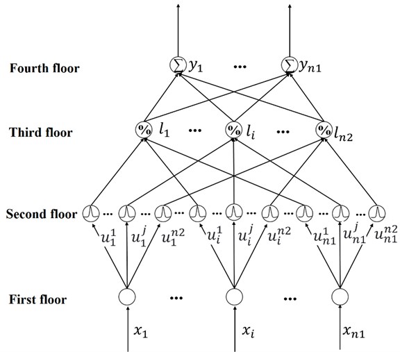
The first layer means the input layer, in which is the input of the FNN, where is the number of inputs.
The second layer is the fuzzy membership degree calculation layer of each input component, using a Gauss function:
where , ; refer to the center and width concerning the fuzzy basis functions (FNNBF) respectively, and the center and width vectors of the basis function are as follows:
Among which .
The third layer is used to match the antecedent of fuzzy rules, the completed calculation is:
The fourth layer means the output layer for clarity calculation:
where means the output of the FNN.
The matrix form of the fuzzy neural network can be obtained as:
where is the output vector, means the weight matrix, and means the output base vector.
3. Controller design
3.1. Control objective
Assuming that the joint rotation angle of the mechanical arm , and the angular velocity of the joint are measurable values, the expected angle and its derivative are given, other parameters of the system are unknown, an adaptive fuzzy neural network controller (AFNNC) is designed, and when to make sure that , .
3.2. Controller design
The angle error is defined as follows:
Then, the angular velocity error is:
And the sliding surface is:
where the constant is an adjustable parameter. The added intermediate variable is defined as:
Taking the derivation of Eq. (11), it yields:
Substituting Eqs. (8-12) into Eq. (1), it yields:
Eq. (13) can be rewritten as:
where is the nonlinear function which includes LuGre friction links. The fuzzy neural network mentioned above is used for approximation:
where and are respectively the ideal weight matrix and output base vector of the FNN, means the approximation error vector, and is the input of the fuzzy neural network. The true value , , is unknown, and its estimated value is , , , the estimated errors are defined respectively as , , , , can be described as:
where , , is the residue.
By combining Eq. (15) and Eq. (16), the approximation error of the fuzzy neural network to nonlinear links is obtained:
where:
Assuming that is bounded, and is an unknown bounded disturbance vector, then vector is bounded, thus there is one active definite diagonal matrix which meets .
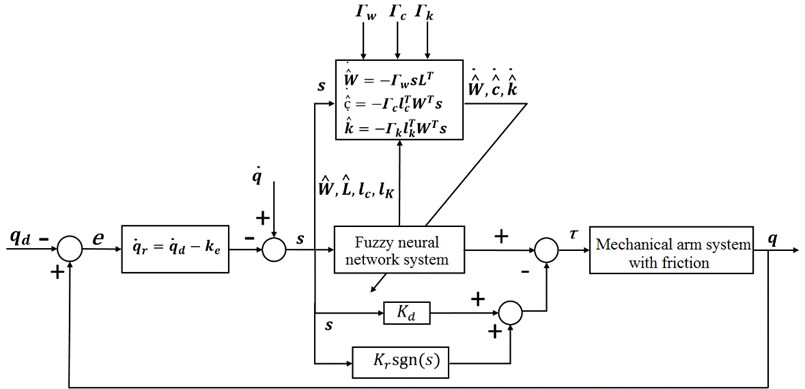
The control rate is taken is:
where and are the positive definite diagonal matrices, is the output of the fuzzy neural network to approximate nonlinear functions . According to Eq. (14) and Fig. 2, is actually a feedforward term. By promptly approximating the unknown nonlinear links, the influence of system nonlinearity can be set to improve the controller’s ability to cope with the unknown nonlinear problems. is the approximation rate, which can suppress the approximation error of the FNN and the influence of unknown disturbance. The parameter self-adaptive law of the FNN is selected as follows:
where , , are the well-dimensional positive definite diagonal matrices.
4. Stability analysis
Theorem 1: For the mechanical arm system where the Eqs. (1) and (3) described, the definition of error is described in Eqs. (8) and (10). The fuzzy neural network controller which is made up of the control rate of Eq. (19), and the parameter adaption rate of Eq. (20), if the conditions of equation are met, the closed-loop system tends to be asymptotically steady.
Substantiation: Taking the Lyapunov function, the following formula is got:
Taking the derivation of Eq. (21), one yields:
Substituting Eqs. (14), (15), and (19), one yields:
According to Eq. (2), substituting Eqs. (17) and (20) into Eq. (23), one yields:
Because of the property:
Therefore:
As for , there is , Eq. (26) can be rewritten as:
Due to ,we get:
As it can be seen from the lemma Barbalat, when , . According to the Eq. (10), and , it is found that and at , the proof is completed.
The framework of the adaptive FNN controller is presented in Fig. 2.
Fig. 2Framework of adaptive FNN controller
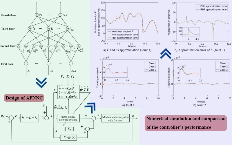
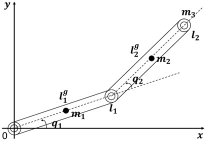
5. Numerical simulation
AFNNC and neural network algorithm (RBF) are compared and simulated in MATLAB2019b environment. The planar two-joint manipulator is taken as the object, and shown in the model view in Fig. 3. Among them, , , and are the masses of two connecting rods and the load respectively, and are the sizes of two connecting rods respectively, and and are the distances of the centroid. The parameters of the mechanical arm are selected as follows: 4 kg, 3 kg, 1 m, 1 m, 0.5 m, 0.5 m; is the joint angle vector of the robotic modulator, and the initial values are taken as: , .
The desired trajectory of the joint angle of the robotic modulator is taken as:
The disturbing moment subjecting the mechanical arm system is taken as:
The parameters within the LuGre Friction model are selected as: 10000 Nm, 35 Nm, 0.2 N⋅m⋅s/rad, 0.3 Nm, 0.45 Nm, 0.005 Nm.
Fig. 3Industrial mechanical arm model of two connecting rods
The parameters of the joint space trajectory tracking controller based on the fuzzy neural network are selected as follows: parameter is related to the steady state accuracy of the system, a large overshoot may occur when the value is too large, thus this number shall take a moderate value; parameter significantly affects the convergence speed of the sliding mode surface and the steady-state accuracy of the system, thus this parameter shall be a large value; parameter can restrain the approximation error of the fuzzy neural network and system disturbance, thus this parameter shall be a moderate value. The specific selection of value is as follows: 10, , .
Since the control quantity contains discontinuous terms , it will inevitably lead to buffeting. In order to suppress buffeting, a hyperbolic tangent function is adopted instead of the symbolic function in the simulation. In the following simulations, all the controller parameters are consistent with the above simulation conditions except for the friction parameter of the LuGre friction model.
is regarded as the input of the FNN. Because of , the number of inputting and outputting layers of the fuzzy neural network is selected as: 2, 2. The number of fuzzy membership functions for each input is which corresponds to respectively.
Since the fuzzy neural network contains parameters , , and self-adaptation rate parameters , , , it is necessary to select appropriate parameters for better controller performance. As a result, the selection of above parameters was first studied.
5.1. Influence of fuzzy neural network parameters on control performance
5.1.1. Influence of initial parameter value
The influence of the initial value of the weight matrix on the control performance is studied firstly. Three sets of simulation for the different initial values are compared in cases of zero load (0 kg) on the mechanical arm, and the friction parameter is constant. Case 1: All elements of are equal to 0; Case 2: All elements of are equal to 10; Case 3: All elements of are set to a random number between 0 and 10. The initial values of the other parameters and the renewal law parameters are the same: , , , where is the appropriate dimensional unit matrix.
The trajectory tracking errors of the mechanical arm in three cases are shown in Fig. 4. In case of the different initial values, the convergence time, overshoot and steady state errors of the system are almost indifferent. It means that the selection of the initial value of the output weight has no obvious effect on the controller performance. The main reason is that can be updated in the real time according to the system response. As a result, the selection of is quite simple. In order to avoid the problem of excessive control amount at the initial time, it is required just to select a relatively moderate value of .
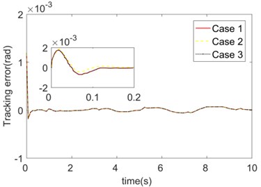
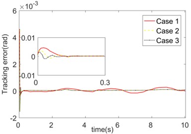
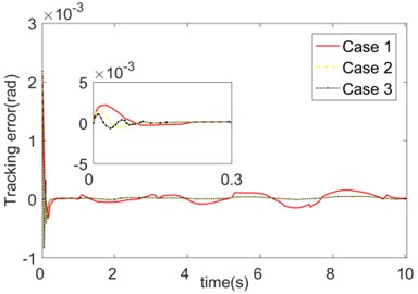
Then the influence of the initial value selection of the basis system function was studied. The simulation cases of the following three different initial values are compared. Case 1: , ; Case 2: , ; Case 3: , 0.5.
Fig. 4Trajectory tracking errors of initial values of different FNN weight matrices
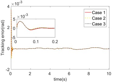
a) Joint 1
b) Joint 2
Fig. 5Trajectory tracking errors of initial values of different FNN fuzzy basis functions
a) Joint 1
b) Joint 2
The trajectory tracking errors obtained in these three cases are shown in Fig. 5. Similar to the various initial value selection of the weight matrices , the initial value selection of the basis function does not differ significantly in controller performance. As a result, compared with the fuzzy logic and other methods, the domain selection in the process of constructing the controller using fuzzy neural network is relatively simple, and only needs to be selected according to the experience. The center and width , of the fuzzy set function can track the system response for online adjustment.
5.1.2. Influence of adaptive law parameters
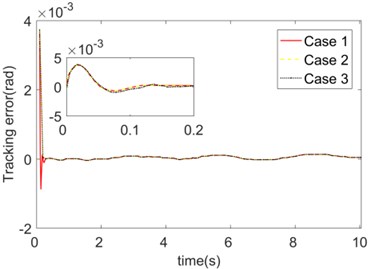
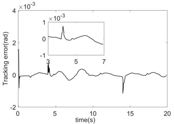
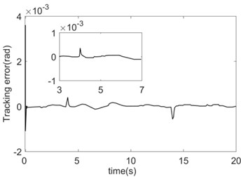
The influence of adaptive law parameters on controller performance was analyzed as follows. Firstly, the different values of are compared and simulated. Case 1: ; Case 2: ; Case 3: . The trajectory tracking errors of the three cases are presented in Fig. 6. The selection of influences both the convergence speed and steady-state errors of tracking. When choosing a smaller value (Case 1), the error convergence is slower, and the steady-state error is larger. The reason might be in that in the control process, too small restricts the approximation performance of the FNN to the unknown nonlinear links. At this time, the fuzzy neural network has a limited ability to deal with nonlinear links. When choosing a larger value (Case 3), the error converges quickly, and the steady-state error is small. But when is too large, a certain overshoot occurs.
Fig. 6Trajectory tracking errors of different FNN updating law parameters Γw
a) Joint 1
b) Joint 2
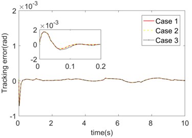
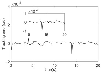
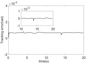
Different adaptive law parameters , of the fuzzy basis function are simulated and analyzed in this paper. Case 1: ; Case 2: ; Case 3: . The trajectory tracking errors of the three cases are presented in Fig. 7. It illustrates that the values of have no significant impact on the steady-state performance, and its influence is mainly reflected in the joint commutation of the mechanical arm and the jumping time of friction force. So, the robustness of the controller to abrupt non-linearity can be improved only by selecting a suitable value of , .
In conclusion, the selection method of the FNN parameters is as follows: In order to avoid the problem of excessive control amount at the initial time, shall not be too large; In the selection process of , , appropriate values can be selected according to the experience; Parameter is related to the approximation performance of the fuzzy neural network to the nonlinear function, as well as to the steady-state error, thus a larger value shall be taken; The selection of parameters , will affect the system robustness to sudden interference, thus a moderate value shall be taken. As a result, the initial values of the FNN can be selected as: , , 1, 2, 1,…,7, and:
The adaptive law parameters can be selected as: , , .
Fig. 7Trajectory tracking errors of different FNN updating law parameters Γc, Γκ
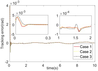
a) Joint 1
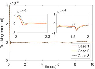
b) Joint 2
5.2. Robust performance
To further verify the tracking performance of the controller, the robust performance of the control strategy and the approximation performance of FNN to the nonlinear function , two algorithms: AFNNC and RBF are compared.
The absolute error integral is set as the error index function: . The function of the system friction coefficient changing with time is: . The initial load is 2 kg; when 4 s the load changes to 3 kg; when 14 s the load changes again to 1 kg. The simulation outcomes are shown in Figs. 8-9.
Fig. 8Comparison of tracking errors between FNN and RBF when friction coefficient is time-varying and load is mutation
a) RBF tracking error (Joint 1)
b) AFNNC tracking error (Joint 1)
c) RBF tracking error (Joint 2)
d) AFNNC tracking error (Joint 2)
The two control strategies are both based on the combination of sliding mode control and compensation for nonlinear link . In order to verify the effectiveness of the algorithm as objectively as possible, the same sliding surface and approach law are adopted for the RBF controller. And the selection of the center and width of the RBF controller’s basis function is the same as the initial value of the FNN basis function parameter. The only difference between the two controllers is that the basis function center and width of RBF are fixed, while the basis function center and width of fuzzy neural network in AFNNC controller can be adjusted online according to the system response.
The tracking errors of the system can both converge quickly under the two control algorithms. However, the convergence speed of the errors under the AFNNC control strategy is slightly faster than that of the RBF controller, and the steady-state error and the error jump at the time of load mutation is also smaller (Fig. 8). Since the two control strategies are compensated by approximating the nonlinear link and the feed-forward, the approximation performance of the nonlinear link affects the control performance directly.
The approximation contrast and error of the nonlinear function of the system using FNN and RBF are shown in Fig. 9. Both compensation strategies can realize the effective compensation of the nonlinear function . When the load jumps 4 s, 14 s, produces the corresponding jumps. (Fig. 9(a) and 9(c)). Since the , of the fuzzy basis function adopted by the FNN can be dynamically adjusted according to the system response, the convergence speed of the FNN approximation error is faster than that of the RBF. Throughout the process, the approximation error of FNN is smaller than that of the RBF (see Fig. 9(b) and 9(d)).
Fig. 9Comparison of compensation effects between FNN and RBF when the friction coefficient is time-varying and load is mutation
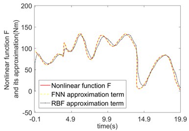
a) and its approximation (Joint 1)
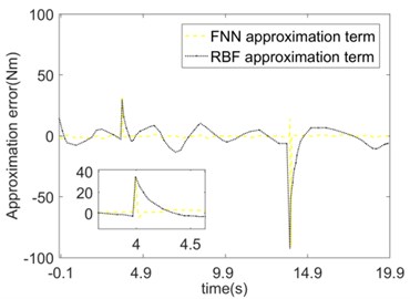
b) Approximation error of (Joint 1)
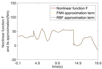
c) and its approximation (Joint 2)
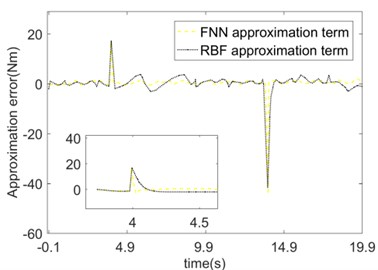
d) Approximation error of (Joint 2)
The error comparison between the two control strategies is shown in Table 1. Benefiting from the good approximation performance of FNN, the tracking accuracy of the system is higher, and the robustness is better when adopting the AFNNC control strategy.
Table 1Comparison of system tracking errors when friction and load change
Tracking error comparison at steady-state and jump time | ||||||
Steady-state error | Jump error when 4 s | Jump error when 14 s | ||||
Joint 1 | Joint 2 | Joint 1 | Joint 2 | Joint 1 | Joint 2 | |
RBF | 2×10⁻⁴ rad | 2×10⁻⁴ rad | 8×10⁻⁴ rad | 5×10⁻⁴ rad | 1.3×10⁻³ rad | 1.3×10⁻³ rad |
AFNNC | 1×10⁻⁴ rad | 1×10⁻⁴ rad | 3×10⁻⁴ rad | 2×10⁻⁴ rad | 0.6×10⁻³ rad | 0.6×10⁻³ rad |
Error index comparison | ||||||
Joint 1 | Joint 2 | |||||
RBF | 2.0263×10⁻³ rad (0.1161) | 1.8644×10⁻³ rad (0.1068) | ||||
AFNNC | 8.6735×10⁻⁴ rad (0.0497) | 5.4568×10⁻⁴ rad (0.0313) | ||||
6. Conclusions
In this paper, the LuGre friction model was introduced into the mechanical arm system. An adaptive fuzzy neural network controller was designed under the condition that the system dynamics parameters were unknown, and the steadiness of the mechanism was proved by Lyapunov method. The simulation results show that the fuzzy neural network can approximate the nonlinear link quickly and accurately. In case of changes in load and working environment, the control strategy proposed in this paper can realize high-precision trajectory tracking of the mechanical arm in the joint space, and it has good robustness to load mutation.
References
-
Marton L., Lantos B. Modeling, identification, and compensation of stick-slip friction. IEEE Transactions on Industrial Electronics, Vol. 54, Issue 1, 2007, p. 511-521.
-
Owen W. S., Croft E. A. Reduction of stick-slip friction in hydraulic actuators. IEEE/ASME Transactions on Mechatronics, Vol. 8, Issue 3, 2003, p. 362-371.
-
Bigras P. Reduced nonlinear observer for bounded estimation of the static friction model with the Stribeck effect. Systems and Control Letters, Vol. 58, Issue 2, 2009, p. 119-123.
-
Márton L., Lantos B. Control of mechanical systems with Stribeck friction and backlash. Systems and Control Letters, Vol. 58, Issue 2, 2009, p. 141-147.
-
Moshkovich A., et al. Stribeck Curve Under Friction of Copper Samples in the Steady Friction State. Tribology Letters, Vol. 37, Issue 3, 2010, p. 645-653.
-
Shang W., Cong S., Zhang Y. Nonlinear friction compensation of a 2-DOF planar parallel manipulator. Mechatronics, Vol. 18, Issue 7, 2008, p. 340-346.
-
Caprino S., Cavallaro G., Marchioro C. On a microscopic model of viscous friction. Mathematical Models and Methods in Applied Sciences, Vol. 17, Issue 9, 2007, p. 1369-1403.
-
Zhong C. W., Xiang J., Wei W., et al. Simple nonlinear observer based dynamic LuGre friction compensation. Journal of Zhejiang University, Vol. 46, Issue 4, 2012, p. 764-769.
-
Min L. I., Wang J., Xiao K., et al. Sliding mode control of robot with dynamic friction and dead zone compensation using fuzzy logic and neural network. Journal of Chongqing University, Vol. 36, Issue 6, 2013, p. 18-25.
-
Yue F., Li X., Cheng C., et al. Adaptive integral backstepping sliding mode control for opto-electronic tracking system based on modified LuGre friction model. International Journal of Systems Science, Vol. 48, Issue 4, 2017, p. 3374-3381.
-
Zhou X., et al. Improved cerebellar model articulation controller based on the compound algorithms of credit assignment and optimized smoothness for a three-axis inertially stabilized platform. Mechatronics, Vol. 53, 2018, p. 95-108.
-
Han S. I., Lee K. S., Min G. P., et al. Robust adaptive dead zone and friction compensation of robot manipulator using RWCMAC network. Journal of Mechanical Science and Technology, Vol. 25, Issue 6, 2011, p. 1583-1594.
-
Sun Y. H., Sun Y., Wu C. Q., et al. Stability analysis of a controlled mechanical system with parametric uncertainties in LuGre friction model. International Journal of Control, Vol. 91, Issue 4, 2018, p. 770-784.
-
Wang X., Wang S. High performance adaptive control of mechanical servo system with LuGre friction model: identification and compensation. Journal of Dynamic Systems Measurement and Control, Vol. 134, Issue 1, 2012, p. 11-21.
-
Zheng Y. Q. Parameter Identification of LuGre friction model for robot joints. Advanced Materials Research, Vol. 479, Issue 481, 2012, p. 1084-1090.
-
Wu X. D., Zuo S. G., Lei L., et al. Parameter identification for a LuGre model based on steady-state tire conditions. International Journal of Automotive Technology, Vol. 12, Issue 5, 2011, p. 671-685.
-
Zhou X., Zhao B., Liu W., et al. Compound scheme on parameters identification and adaptive compensation of nonlinear friction disturbance for the aerial inertially stabilized platform. ISA Transactions, Vol. 67, 2017, p. 293-305.
-
Zhi Hao X.-U., Sheng L. I., Zhang R. L., et al. Fuzzy-neural-network control for robot manipulators with LuGre friction model. Control and Decision, 2014, p. 493-505.
-
Khayati K., Bigras P., Dessaint L. A. LuGre model-based friction compensation and positioning control for a pneumatic actuator using multi-objective output-feedback control via LMI optimization. Mechatronics, Vol. 19, Issue 4, 2009, p. 535-547.
Cited by
About this article

Supported by the Science and Technology Innovation Projects of Higher Education Institutions in Shanxi (No. 2019L0934). Supported by the Academic Science Foundation of Taiyuan Institute of Technology (No. 2018LG01). Supported by the Academician Workstation of Taiyuan Institute of Technology (TYSYSGZZ201903).
