Baseline-free damage identification based on asymmetrical energy consumption

Ye, Fei; Wu, Jiaquan; Ma, Kun

doi:10.21595/jve.2020.21250

Journal of Vibroengineering

Browse Journal

Submit article

Published: 15 August 2020

Check for updates

Baseline-free damage identification based on asymmetrical energy consumption

Fei Ye¹

Jiaquan Wu²

Kun Ma³

¹Faculty of Civil Engineering and Mechanics, Kunming University of Science and Technology, No.727 South Jingming Rd., Chenggong District, Kunming, 650500, P. R. China

^{2, 3}Faculty of Science, Kunming University of Science and Technology, No.727 South Jingming Rd., Chenggong District, Kunming, 650500, P. R. China

Corresponding Author:

Kun Ma

Cite the article Download PDF

Downloads 967

Abstract

In order to solve the problem of obtaining accurate data for an intact beam, a baseline-free damage identification approach, based on the difference in the energy consumption of a beam, has been presented in this paper. An energy model was established in order to illustrate that the difference in the energy consumption is mainly due to the respiration effect of cracks, and that the energy consumption of a beam bending downward can be utilized as a replacement for the baseline data. Thus, the standard data and the comparative data can be separated from the measurement data. Based on this data, a statistical damage factor that can be used to locate and quantify the damage in a beam has been defined. Finally, an identification algorithm was established and has been experimentally verified for use with pre-damaged reinforced concrete beams. The experimental results have illustrated that the location and singularity of a singular point in the damage indicator sequence can locate the damage and quantify the severity of the damage in a beam, respectively.

Baseline-free damage identification based on asymmetrical energy consumption

Highlights

A baseline-free damage identification method based on asymmetrical energy consumption was proposed and experimentally verified.
The proposed method can locate the damage and quantify the severity of the damage in a beam.
The proposed method can effectively detect the breathing crack in the reinforced concrete beam.

1. Introduction

A crack in a beam is a common and primary form of damage that is responsible for the beam’s initial breakdown, and can seriously degrade its structural health and the in-service lifetime of an entire bridge. In this context, a method to efficiently identify damage in beams and monitor the structural health of bridges has become an important yet timely topic in the field of bridge engineering [1-3].

Generally, one common method that is used to identify any possible damage in beams is to collect their dynamic characteristics, e.g., the frequencies, mode damping, and the modal shapes of the beam based on vibration, and then to achieve identification of the damage by making a direct comparison with characteristics extracted from undamaged beams. It is obvious that the prerequisite for this strategy is easily-accessible modal parameters, namely the baseline data, of intact beams; acquiring this data is still a challenge given the huge number of beams that are used in the engineering field [4]. In order to overcome this problem, a reference state can also be theoretically derived from a finite element model. However, the inappropriate application of FEM inevitably results in the reference state deviating considerably from those measured in the intact state, this reducing thus the reliability of vibration-based damage identification methods. Therefore, it is highly necessary to develop a new damage-identification method on the condition of vanishing baseline data [5].

As early as 1996, an attempt [6] was made to utilize the experimental modal data and modal parameters of the finite element model in order to estimate the base-line modal parameters, and conducted damage localization research on a continuous beam. Later, using the gapped smoothing method, [7] a reference state was constructed in the literature by fitting the curvature mode shape and locating a delamination in a composite beam; based on this method, the damage in the metallic splint-core of a truss structure could be detected with reasonable accuracy [8], fully indicating that damage identification can be achieved even without baseline data. By replacing the curvature of an ideal beam with smoothed polynomials, [9] a non-baseline method for damage identification in plate structures was also reported in the literature. Moreover, by strongly relying on the nodal characteristics of different modal shapes, [10] a reference state for non-baseline damage identification was established; this method could also be used to locate the damage as well as quantitatively evaluate it. Baneen et al. [11]improved the existing modal strain energy method by minimizing the effect of noise on the measurement data. A baseline-free damage identification process of a steel beam was carried out with the modification of using a fitted curvature. Prawin et al. [12] utilized the nonlinear harmonics and inter modulations in the response to establish a damage indicator based on singular spectrum analysis. They also carried out numerical simulation and experimental studies to detect a breaking crack, as well as localization and characterization using singular spectrum analysis. Qiu et al. [13]obtained the health information of a beam by comparing pitch-catch pairs with different propagation distance. Based on distance compensation, they illustrated a damage identification approach for plate-like structures. In 2019 [14], a non-baseline method was reported for identifying damage in a truss by integrating displacement and strain measurements. Han et al. [15] proposed a baseline-free sparse array system based on the fundamental shear horizontal (SH0) wave. This system was used for damage identification of isotropic plates. Randhawa et al. [16] obtained the curvature mode shape using the finite difference of the displacement mode shape, and then obtained the data of an intact beam by smoothing the finite difference approximation with cubic polynomials. The key aim of these studies was the use of a specific algorithm to manually establish a proper reference state; in order to make the reference data algorithm-dependent and deviate from the realistic characteristic of a structure. Thus, in order to improve the accuracy and reliability of non-baseline damage identification, establishing a reference state from the as-measured dynamic signal is highly desirable.

In this work, a non-baseline data method for damage identification has been reported, based on an energy-consumption model. By applying this method to several deliberately damaged beams, it has been demonstrated in this paper that the proposed method can correctly identify the properties of the as-made damage in the beams, thus providing a reliable method for damage identification in a beam structure on the condition of vanishing standard baseline data.

The rest of this paper has been organized as follows: In Section 2, an explanation of the energy- consumption model and damage identification, without baseline data, has been given, the specific experiment has been detailed in Section 3, and finally the paper has been summarized in Section 4.

2. The theory of damage identification without baseline data

2.1. Replacement of the baseline data

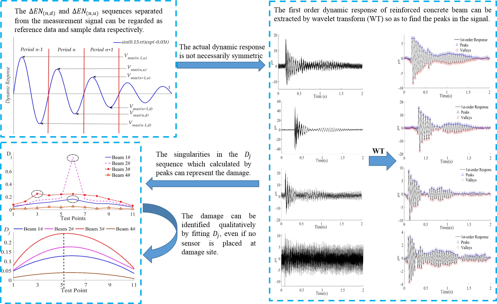
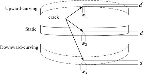
The fundamental principle of the proposed method to identify a breathing-crack in a damaged beam has been schematically illustrated in Fig. 1. In a static state, a crack in a damaged beam which is slightly bent due to gravity has a finite width $w_{2}$ and depth $d$ ; when the beam curves downward, the crack tends to open due to the tensile force acting on it and displays an enlarged width $w_{3}$ . Considering that the severity of the damage of the beam will not significantly change instantly without strong external excitation, the crack depth $d$ can be approximately regarded to be a constant. Conversely, when a beam curves upward, the compressive force tends to gradually cause the crack to close, displaying a shrinking width $w_{1}$ and crack depth $d'$ . The value of $d'$ will decrease as the upward-curving amplitude increases: it will be greater than 0 and less than $d$ . Obviously, the crack width in these cases satisfies the relation $w_{1} < w_{2} < w_{3}$ . Thus, through a single measurement, in contrast to the symmetrical dynamic characteristics of an intact beam, an asymmetrical dynamic characteristic should be expected for a damaged beam. Specifically, due to the barely varying value of $d$ , a relatively stable characteristic can be expected for a downward-curving beam; while for an upward-curving beam, the varying crack depth results in a varying response from the damaged beam. Following this feature, it may be feasible to construct a reference state for non-baseline identification by employing the stable dynamic characteristics of a downward-curving beam and achieve damage identification by taking the response of an upward-curving beam as the control case.

Fig. 1Schematic diagram of the bending shape of a beam

2.2. Energy-consumption model and damage indicator

In order to search for a specific damage indicator, the transverse damped vibration of an Euler-Bernoulli beam should be considered; the system’s energy $E N$ , based on the law of the conservation of energy, can be written as:

1

E N = V_{m a x} + W_{d},

where, $V_{m a x}$ is the maximum potential energy, $W_{d}$ is the energy consumed by the work due to the damping reflection. $V_{m a x}$ can be given as [17]:

2

V_{m a x} = \frac{1}{2} A^{T} K A,

where, $A$ is the modal shape, $T$ denotes the transpose of the matrix, $K$ is the stiffness of the system. For intact beams, the stiffness $K$ is a constant; however, for damaged beams, the stiffness not only decreases but is also variable. A schematic diagram of the local stiffness of a damaged beam with a breathing-crack is shown in Fig. 2.

Fig. 2Schematic diagram of the dynamic response attenuation and energy of a beam

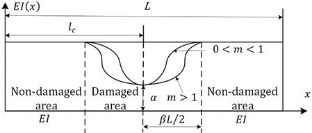
The stiffness expression can be given in another form [18] as:

3

E I (x) = E_{0} I (1 - s α {c o s}^{2} (\frac{π}{2} {(\frac{|x - l_{c}|}{\frac{β L}{2}})}^{m})), (l_{c} - \frac{β L}{2}) < x < (l_{c} + \frac{β L}{2}),

where, $E$ ( $E_{0}$ ) is the Young’s modulus of the damaged (intact) beams, and $I$ is the moment of inertia, $E I$ ( $E_{0} I$ ) is the stiffness of the beam in a damaged (intact) state, $L$ is the length of the beam, $m$ describes the trend of the Young’s modulus in the damaged area of the beam, $x$ is the local position coordinate, $l_{c}$ is the position of the center of the crack, $α$ is the degree of damage with the value range from 0 (intact beam) to 1 (completely broken beam), $β$ is the area affected by the damage with the value range from 0 (no affect) to 1 (the entire beam is affected), and $s$ is the degree of crack closure with the value range from 0 (the crack is completely closed) to 1 (the crack is completely opened). Since the vibration of the beam is generally elastic, for an intact beam, $s$ is always 0 before any cracks appear. For a beam with a breathing-crack, if the beam curves downward, $s$ will always be 1. Correspondingly, if the beam is bent upward, $s$ will be less than 1 and will be time-varying.

Given the contribution of any possible damping, the energy of the beam should be gradually attenuated. In order to see more clearly what could be expected from this feature for damage identification, the way in which the concept of the attenuation coefficient is introduced has been borrowed here [17]. A representatively attenuated response (e.g. displacement) has been plotted in Fig. 3 by taking the expression $f = s i n (0.15 π t) e x p (- 0.03 t)$ as an illustrative example.

Fig. 3Schematic diagram of the attenuated dynamic response and the maximum potential energy of a beam

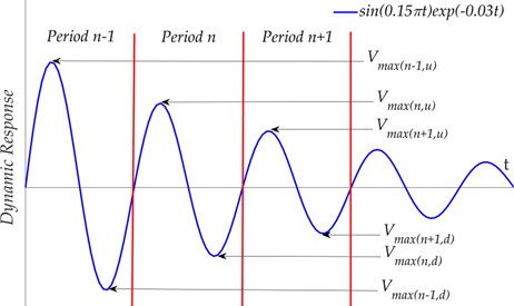
It can be easily seen that as $t$ increases, a series of peaks and valleys can be observed and, due to the damping, the amplitude of these peaks and valleys are different from time to time. At the peaks, the beam is curved upward and acquires a local maximum upward bend; while at the valleys the beam is curved downward and also acquires a local minimum downward bend. For a given periodic value of $n$ , the strong deformation at the peak or valley gives rise to a local maximum potential energy $V_{m a x (n, u / d)}$ with the subscript $u / d$ for the upward or downward curving. It is evident that, due to the damping, there is an observable difference in two neighboring values $V_{m a x (n, u)}$ ( $V_{m a x (n, d)}$ ). Here the energy consumption $∆ E N$ can be used to describe this difference, which can be given as:

4

{∆ E N}_{(n, u / d)} = V_{\max (n, \frac{u}{d})} - V_{\max (n + 1, \frac{u}{d})} .

For a homogenous, intact beam, the asymptotic line of the peaks and valleys is symmetrical with respect to the zero-line and ${∆ E N}_{(n, u)}$ should have little difference from its downward curving counterpart; e.g., the external damping arising from the damper. However, for a damaged beam, there is an observable difference between ${∆ E N}_{(n, u)}$ and ${∆ E N}_{(n, d)}$ due to the respiration effect of the internal cracks. This can be explained by the change in the stiffness of the beam. According to Eq. (3), since the value of $s$ is always 1 when the beam curves downward, the stiffness can be regarded to be constant; while the stiffness of the beam is time-varying due to time-varying value of $s$ when the beam is bent upward. As a physical parameter that reflects the bending performance of the beam, the change in the stiffness will affect the transverse displacement of the beam when it vibrates. The change in the maximum lateral displacement of the system determines the change in the maximum potential energy of the system, which reflects the change of the system’s energy. That is to say, the difference between the stiffness of the beam in different bending states is positively correlated with the change in energy during adjacent periods. In the following section, this difference between the $n$ -th periodic and the $(n + 1)$ -th periodic has been denoted as $ε_{n}$ , which can be written as:

5

ε_{n} = |{∆ E N}_{(n, u)} - {∆ E N}_{(n, d)}| .

For an intact beam, the value of $ε_{n}$ should be zero; while for a damaged beam, a non-zero value would be expected. In addition, in order to reduce the effect of any possible error on $ε_{n}$ and considering the instability of the dynamic response, the statistically averaged value of $ε_{n}$ has been employed here as the damage factor $D_{j}$ for each test point (see Fig. 4(a)), given by:

6

D_{j} = \sqrt{\frac{\sum_{i = 1}^{i = n - 1} {(ε_{i})}^{2}}{n - 2}},

where, $j$ is the order of the test points. Starting with Eq. (6), it can be concluded that a larger value of $D_{j}$ should be observed, due to the position-dependent stiffness, for the test points that more closely approach the center of the crack. Due to the respiratory effect of the crack, a larger value of $D_{j}$ with a specified test point should also be observed for the asymmetry of a much larger energy consumption. It should be noted that: (1) according to Fig. 2, only the local stiffness in the damaged area is reduced, therefore only the data that is detected by the test points in the damaged area is able to reflect the damage; (2) in the damaged area, the stiffness of the area close to the center of the fracture is significantly decreased, while the stiffness of the area far away changed much less noticeably. Therefore, the sensitivity of the data that was obtained from the test points in the region that was relatively far away from the damage is relatively weak. Thus, according to the analysis of $D_{j}$ , the damage can then be located and evaluated.

3. Experimental study on pre-damaged reinforced concrete beams

3.1. Artificially cracked reinforced concrete beams and the measurement system

The experiments were conducted on four reinforced concrete beams with dimensions of 600 cm × 25 cm × 50 cm; three of the beams were prefabricated with artificial cracks and all the beams were simply supported. The density of the beams was 2.5×10³ kg/m³ and the thickness of the concrete cover was 4 cm. Each beam had two pressed longitudinal stirrups and three tensioned longitudinal stirrups with a diameter of 2 cm. The diameter and configuration spacing of the stirrups were 0.8 cm and 20 cm respectively. The stirrup grade, the concrete’s compressive strength and the elastic modulus were HRB335, 32 MPa and 30 kN/mm², respectively. The structural schematic diagram of the beams and the details of the artificial cracks have been shown in Fig. 4 and Table 1 respectively.

Table 1Details of the test specimens

	#1 Beam	#2 Beam	#3 Beam	#4 Beam
Crack location	Mid-span	Mid-span	A quarter of the beam’s length	No damage
Crack depth (cm)	2.5	10	2.5	0

Fig. 4Structural diagram and images of the reinforced concrete beam

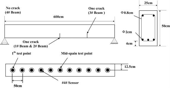
a) Structural diagram and distribution of the test points on the beam

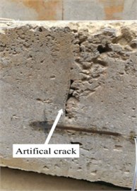
b) Artificial crack

c) Reinforced concrete beam

In order to record the dynamic response of the beam to an external shock, an array of sensors was evenly arranged in a line at the bottom of the beam from one end to the other, as shown in Fig. 4(a). The purpose this layout was to verify the feasibility of using this method in one-dimensional simple structure damage identification. A total of 11 sensors were set up on each beam. The distance between two adjacent sensors was 50 cm, and the distance between the two boundaries is 12.5 cm. Each sensor contained two strain gauges; one was the measuring instrument and the other was the compensator. The parameters of the strain gauges are shown in Table 2.

Table 2Parameters of the BX120-100AA strain gauge

Resistance value	Length and width of the base	Length and width of the wire grid	Supply voltage	Sensitivity coefficient	Strain limit
120 Ω	108 mm×6 mm	100 mm×3 mm	3 V-10 V	2.0 ± 1 %	20000 με/m

The initial non-zero strain, caused by the self-deformation of the beam, and other random factors can be eliminated by initialization of the test system. In other words, when the beam is static, the strain measured at all test points was set to 0.

Since it is very difficult to produce a real breathing crack in a beam, artificial cracks (shown in Fig. 4(b)) were simulated by the manual addition of a piece of cardboard at a specific location when the beam was manufactured. As the coupling between the concrete and the cardboard is weaker than that between concrete and concrete, the tensile stress on the cardboard will be significantly reduced (even to 0) when the beam curves downward. From the point of view of a stress state, the damage produced is similar to that of an actual breathing-crack. Conversely, when the beam curves upward, the concrete on either side of the cardboard can be considered to be in approximate direct contact as the cardboard is very thin. Therefore, it is expected that the experimental data obtained from this setup can reasonably represent the damage in a beam with an actual crack. The length and thickness of the cardboard that was used was 25 cm and 0.05 cm respectively. By artificially imposing an external shock with a 10 kg hammer (as shown in Fig. 4(c)), a random impulse excitation was simulated in order to eliminate the interference of an external force on the energy consumption caused by the damping and ensure that the as-measured dynamic response would be recorded in-situ by a computer.

3.2. Damage identification based on the 1st-order dynamic strain response

3.2.1. Extraction and separation of the dynamic response

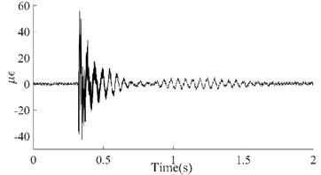
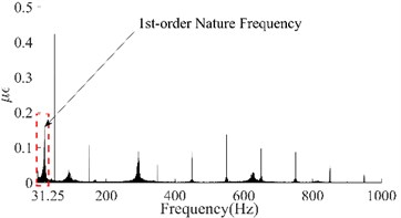
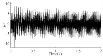
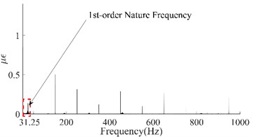
Taking the dynamic response that was measured from the 6th test point of the #1# beam as an example, Fig. 5(a) depicts the as-measured signal from the #1 beam. It can be easily observed that the signal showed a certain asymmetry with respect to the zero-line; the maximum value of the peaks was approximately 17 while the minimum value of the valleys was approximately -12. In addition, the roughness of the signal waveform makes the periodicity difficult to ascertain. In order to distinguish the dynamic response components of the signal, firstly the spectrum (as shown in Fig. 5(b)) was obtained using the Fast Fourier Transform of the signal. In Fig. 5(b), a series of spectral peaks can be seen in the spectrum, which can be divided into two categories; ones with a Gaussian Shape and others with a pulse shape. Among these peaks, the pulsed peaks showed a remarkable regularity, that is, their frequencies were all integer multiples of 50 Hz. This indicates that these components were harmonic noise and had to be eliminated before the following analysis was carried out. It was obvious that the remaining peaks represent the natural frequencies that corresponded to each order of the vibration signals. Similarly, the dynamic response that was measured from the 6th test points and their spectrums for beams #2, #3 and #4 have been demonstrated in Fig. 5(c) to Fig. 5(h). Among these, the signal quality for beam #2 was the best (as shown in Fig. 5(c)) due to the weaker harmonic component (as shown in Fig. 5(d)). However, the characteristic of the signal’s asymmetry (maximum 60, minimum 40) cannot be concealed by either the periodicity or the relatively smooth waveform. In contrast, the signal in Fig. 5(g) was the most cluttered, although the symmetry of the amplitude was good. Compared with the spectrum in Fig. 5(h), it is not difficult to see that the clutter in the signal was mainly caused by interference from excessive harmonic noise. The rest, both the response and the spectrum characteristics of beam #3 were all similar to those of beam #1. According to the figures above, the dynamic responses of the three beams, in total, have shown a certain asymmetry; and the beams where this occurred happened to be the damaged beams. This result seems to confirm the above mentioned inconsistency in the vibration of the damaged beam; in both the upward-curving and downward-curving beam. However, whether this inconsistency is due to an intrinsic dynamic response or interference from noise will need to be confirmed by further work. Due to the coexistence of multiple-order vibration signals and the interference from the harmonic noise, the as-measured signal displayed a complex pattern. Directly identifying any underlying damage from this date is a challenge. In general, in order to obtain the intrinsic dynamic response components from the complex signals to allow for subsequent analysis, a filter is needed. In view of the complexity of the traditional design of a filter and the feasibility of damage identification using the 1st order signal [19], wavelet decomposition was carried out in this paper.

Due to the irregular shape of the spectrum peak (as illustrated in the subfigure of Fig. 5(d)), it is difficult to determine the bandwidth of each order of the natural frequency. Therefore, the common binary wavelet decomposition was employed to extract the intrinsic signal based on the wavelet toolbox in MATLAB. Based on the fact that the 1st-order signal possesses the most energy of the complete dynamic response signal [20, 21], the target extracted through wavelet decomposition was determined to be the 1st-order signal. According to the principle of binary wavelet decomposition [22], the Frequency Range, $F R$ , of each node can be obtained from Eq. (7):

7

F R = 2^{- k} F_{s},

where, $k$ is the order of decomposition and $F_{s}$ is the maximum analytical frequency. According to Fig. 5, the 1st-order natural frequencies of the four beams were 21.52 Hz, 19.6 Hz, 20.97 Hz and 23.45 Hz respectively. As the maximum analytical frequency of all the four group signals were 1000 Hz, it was necessary to perform a five-layer decomposition to extract the 1st-order signals. After decomposition, the frequency range of the approximate nodes was 0 Hz-31.25 Hz (Highlighted with a red dotted box in the figures). Obviously, the signal in the approximation node was the 1st-order response; this is because the waveform of the signal that is obtained by wavelet decomposition is related to the basic wavelet. In order to obtain a signal that is as smooth as possible and facilitate extraction of the peaks, the DB6 wavelet with good smoothness was selected as the basic wavelet during decomposition. The four 1st-order signals have been illustrated in Fig. 6.

Fig. 5Dynamic response and spectrum of the 6th point on each of the four beams based on the strain measurement

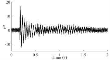
a) Dynamic response of the #1 Beam

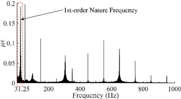
b) Spectrum of the #1 Beam

c) Dynamic response of the #2 Beam

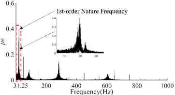
d) Spectrum of the #2 Beam

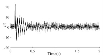
e) Dynamic response of the #3 Beam

f) Spectrum of the #3 Beam

g) Dynamic response of the #4 Beam

h) Spectrum of the #4 Beam

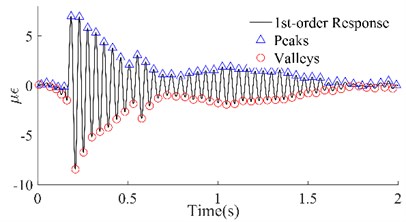
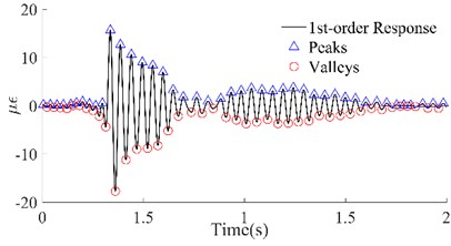
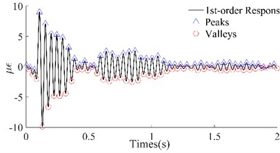
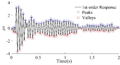
Fig. 61st order responses and peaks/valleys array of the four beams

a) #1 Beam

b) #2 Beam

c) #3 Beam

d) #4 Beam

In Fig. 6, the 1st-order responses (black lines) that were extracted by wavelet decomposition have been shown, which not only separated the other order responses but also filtered out the harmonic noise, compared with the original dynamic responses. Among them, the improvement in the signals of beams #1 and #2 was the most significant, while that of beams #3 and #4 was slightly worse. Although the local signals for beams #3 and #4 were chaotic, on the whole, the four group signals were smoother and periodic. According to the attenuation trend of the signals, it is not difficult to see that the reason for the local clutter was the occurrence of multiple hits in one excitation. However, this did not affect the identification of the peaks and valleys which were utilized to calculate the maximum potential energy. The triangles and circles in Fig. 6 are the series of peaks and valleys that were identified with the maximum or minimum in every 50 data points. Although there was still some asymmetry between the sequences of the peaks and the sequences of the valleys of these four beams, it was no longer apparent. The results illustrated that, on the one hand, the signals obtained through wavelet decomposition can truly reflect the intrinsic vibration of the beams, and on the other hand, these beams have potential damage according to the previous inference.

3.2.2. The replacement of potential energy and damage identification

Since the potential energy cannot be calculated from the strain data, the wavelet energy was chosen as an alternative to determine the energy of the system. The wavelet energy $E_{w}$ can now be given as [23]:

8

E_{w} = \int_{- \infty}^{+ \infty} f^{2} (t) d t .

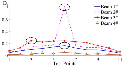
Eq. (8) describes the energy of one wavelet node. Therefore, the maximum potential energy $V_{m a x (j, u / d)}$ was calculated from the sequence of the peaks and valleys. The damage indicator $D_{j}$ was obtained by substituting the data from the sequences of the peaks/valleys into Eq. (8), Eq. (5) and Eq. (6). The calculated values of $D_{j}$ of the four beams based on the 1st-order response have been depicted in Fig. 7.

In Fig. 7, the blue curve denotes the value of $D_{j}$ for beam #1. All the eleven values of $D_{j}$ were greater than 0, among which, $D_{6}$ was the largest while the others successively decreased with the increase of the distance from the 6th point. This illustrates that there were differences in energy consumption at all eleven test points and that the consumption at the 6th point was most significant. According to the inference introduced in section 2, this indicated that the crack was located near the 6th test point. The purple curve denoting the $D_{j}$ of beam #2, shown in Fig. 7, is similar to the blue curve. The main difference between them is that not only is the $D_{j}$ on the purple curve larger than that on the blue curve, but also the $D_{6}$ of beam #2 was significantly larger than that of beam #1. This suggests that a crack also exists near the 6th point on beam #2, and the depth of the crack is greater than that in beam #1. The $D_{j}$ of beam #3 is denoted by the red curve. In the red curve $D_{3}$ displayed an obvious singularity which was greater than all the other $D_{j}$ . In addition, the curve formed by the other $D_{j}$ took the shape of an arch. The reason for the arch is that the amplitude of the beam at its mid-span is the largest in general. This feature is further amplified by the square effect when calculating the wavelet energy. However, the arched distribution of the difference in the energy consumption cannot conceal the abnormal increase of the local energy consumption caused by the change in the local stiffness. Therefore, the singularity of $D_{3}$ indicates that a crack appeared near the 3rd point on beam #3. As the singularity of this $D_{3}$ is close to that of $D_{6}$ on beam #1, this indicates that the crack depth in beam #3 is close to that of beam #1. Differing from the first three curves, although the $D_{j}$ on the brown curve of beam #4 are all greater than 0, they are all small values and some are close to 0 (e.g. $D_{1}$ , $D_{8}$ and $D_{11}$ ). The arched feature of this curve is not obvious; this indicated that the difference in the energy consumption of each point is very small. These characteristics indicate that there was no crack in beam #4. By comparing the details in Table 3, these identification results obtained from the information of the four curves have been proved to be true. On the other hand, according to the position of these singular points, the cracks have been located.

Fig. 7Dj curves of the four beams based on the 1st order responses

Therefore, because the singularity of a singular point can reflect the severity of any damage, if the singularity is reflected by the Relative Error (RE) between the singular points and the standard points, the RE can also quantify such damage. Eq. (3) and the curves in Fig. 7 have all illustrated that the local characteristics of the damaged beam near the end point are consistent with that of a healthy beam. Since the 11th points on all of the three damaged beams were all the points that were farthest away from the singular points, the $D_{11}$ were selected as the standard with which to compare with that of the singular points in order to evaluate the damage. The quantitative results have been listed in Table 3.

Although the local properties near the endpoints of the beam are considered to be approximately equal to that of a healthy beam; however the three $D_{11}$ show a significant difference in Table 3. On the one hand, this difference is due to the inconsistent excitation intensities, and on the other hand, it is because of the different intrinsic characteristics of the beams caused by an error (e.g. the uniformity of the concrete, a variable curing environment, etc.) during production. Surprisingly, the REs of beam #1 and beam #3, which were 3.1 and 2.9 respectively, were close (a difference of only 0.2). While, the RE of beam #2, which was 13.2, was about 4 times as large as those of beams #1 and #3. The relationship of these REs is consistent with that of the depths of the cracks in the three beams. Considering the possible errors that have been mentioned above, this result reasonably indicates that damage can be quantified by utilizing the method that has been described in this paper.

Table 3The details of the quantitative evaluation

	$D_{j}$	$D_{11}$	RE
#1 Beam ( $j = 6$ )	0.1661	0.03967	3.1
#2 Beam ( $j = 6$ )	0.8192	0.0575	13.2
#3 Beam ( $j = 3$ )	0.2462	0.06347	2.9

3.2.3. Discussion on the distribution of the test points

The experimental results in the previous section have shown that the method that has been proposed in this paper is able to better identify the damage in a beam. However, in this experiment, one of the measuring points was located at the exact point where the crack was; in the real world this would not be possible. In this section, in order to discuss the influence of the distribution of the test points on the identification results, the data from the special test points (the test points at the damaged region) in the previous experiment have been deleted in order to simulate unknown damage; this will verify the applicability of the baseline-free damage identification method. The data that was deleted originated from the 6th point of both beam #1 and beam #2, and the 3rd point of beam #3. According to the curve of the local stiffness in Fig. 2, the change in the local stiffness is continuous; therefore, the change in the difference of the energy consumption at the different positions should also be continuous. Obviously, the data obtained from limited discrete test points cannot accurately reflect the continuity of the changes in $D_{j}$ . Therefore, curve fitting was chosen as a common method that can be used to solve this problem. Using MATLAB’s “Curve Fitting” toolbox, the $D_{j}$ of the four beams were fitted with a 4th-order polynomial. The fitting curves are shown in Fig. 8:

Fig. 8Fitted Dj curves of the four beams based on the 1st order responses

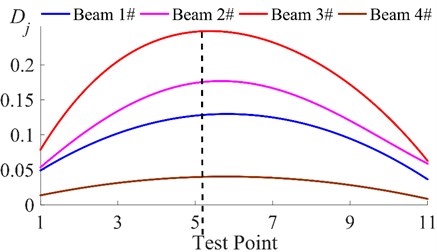
In Fig. 8, all four curves appear arched, which is similar to the result in Fig. 7. However, the curvature of each line is significantly different. Among the four curves, the curve with the least obviously arched feature is the $D_{j}$ fitting curve of beam #4 (brown line). The peak of the brown curve appears near the 6th point, and its maximum value is about 0.04, which is very close to 0. The brown curve, centered on the 6th point, shows good symmetry and the whole curve is very close to being a straight line. These characteristics have illustrated that the differences in the energy consumption at a single point are very small and the differences in the energy consumption at the different points are very close. This result indicates that there is likely no damage in beam 4. The curves of beam #1 (blue curve) and beam #2 (purple curve) both show an obvious arch. Their similarity lies in the peaks all appearing near the 6th point, with the peak point as the center of the graph; the curves on both sides also show good symmetry. The shapes of the two curves indicate that: (1) there are significant energy consumption differences in these two beams, which indicates that both beams may be damaged; (2) the difference in the energy consumption at a symmetrical position on both sides of the 6th point shows good symmetry, indicating that the damage may have occurred near the 6th point. The difference between the two curves lies in their different bending characteristics, with the curve of beam #2 (purple line) having greater curvature. This indicates that the difference in the energy consumption of a single point on beam #2 is larger and the variation in the energy consumption between the different points is more obvious; therefore, the damage in beam #2 is more severe than that in beam #1. The most obviously arched curve is the $D_{j}$ curve of beam #3 (red line). The peak of the red line appears near the 5th point, which indicates that the damage to beam #3 may occur near the 5th point. However, unlike the other three curves, the curves on both sides of the red curve, centered on the black dotted line (near the 5th point), have obvious asymmetry. Among them, the curve to the left of the black dotted line decays faster, indicating that the location of the damage is to the left of the 5th point. Although there is an error between this result and the result from the previous section, this result is acceptable, considering that the data of the test point nearest to the damage has been deleted. Since the identification results of the other three beams are basically the same as those in the previous section, the damage location and damage evaluation can be found qualitatively by using this approach, even if no test point is located at the damaged region. Due to the deletion of the data from the specific test points, there are no obvious singularities in the three curves of the damaged beams (Beam #1, Beam #2 and Beam #3) in Fig. 8. The data from the points (peaks) with the maximum curvature in the curves were used as a substitute for the data from the singularities for quantitative analysis. The relevant data have been listed in the Table 4.

Table 4Quantitative evaluation without obvious singularities

Beam	$L_{p}$	$D_{p}$	$D_{11}$	RE
#1	5.925	0.1296	0.03628	2.6
#2	5.623	0.1767	0.05876	2.0
#3	5.171	0.2478	0.06264	3.0

In Table 4, $L_{p}$ and $D_{p}$ denote the location and the $D_{j}$ of the peaks on the curves in Fig. 8, respectively. The $L_{p}$ of beam #1 and beam #2 are 5.925 and 5.623, respectively, which are close to 6. This indicates that the damage in the two beams is near the 6th point. However, they all have smaller values of RE than those in Table 3. Among them, the RE of beam #1 is 0.5 smaller, while the RE of beam #2 is 11.2 smaller than those in Table 3; therefore, the results of the damage quantification are not reliable. The $L_{p}$ of beam #3 is 5.171; this indicates that the damage may be near the 5th measuring point. There is an error between this result and the result in the previous section; the RE of beam #3 is 3.0, and the error of the results in Table 3 is only 0.1. The above results show that there is an error in the damage quantification results in the absence of measurement data taken near the crack. The reasons for this error may be as follows: The degree of damage from an artificial crack is relatively weak; therefore, affected by this, the area with an obvious change in stiffness is also relatively small. However, after deleting the singularity data, the gap was 50 cm away from the nearest test point. Therefore, the difference in the energy consumption at the test point on the beam is relatively small and its variation trend is relatively slow in the measured area. Based on the above reasons, it can be found from a re-analysis of Fig. 8 that the curves of the three damaged beams are significantly higher than the curve of the healthy beam. This indicates that the existence of an artificial crack reduces the stiffness of the entire beam. This results in a difference in the energy consumption at each test point. The disappearance of the obvious singularities indicates that the region in which the local stiffness significantly decreases is relatively small. It is precisely because there is no sensor in this region that the quantitative analysis error increased.

Based on the above analysis, it is not difficult to reach the following conclusions: (1) It is possible to qualitatively identify the actual damage in a beam, even if there are only a few test points; (2) Based on the results of the qualitative identification, the problem of the increasing error in the quantitative identification can be effectively solved by adding test points to the potentially damaged area. This is also a common method for solving the problem of insufficient measurement quantity that occurs in many existing identification methods. (3) Although the method of increasing the measurement points increases the workload during the detection process, this task is obviously easier to carry out than it is to obtain baseline data.

4. Conclusions

In order to solve the problem of obtaining accurate baseline data of a healthy beam in practical detection, an energy consumption model-based damage identification method, without baseline data, has been proposed in this paper. According to the characteristic where a damaged beam with a breathing-crack has different damping values in different bending states, it can be concluded that the energy variation data of the beam in a downward-curving state can be utilized as a substitute for the baseline data. Based on this conclusion, a statistical damage indicator $D_{j}$ has been defined and then used for experimental verification. The identification results have illustrated that the elements in the $D_{j}$ sequence, based on the dynamic response of the damaged beam, are all greater than 0, while that of the healthy beam approaches 0. The singular point in this sequence means that there is a potential breathing crack near the measurement point. The position of the singular point in the $D_{j}$ sequence means that there is a potential breathing-crack near the corresponding test point, and the singularity of this point quantitatively indicates the severity of the damage in the damaged beam. Although the lack of measurement points near the damaged area can increase the error of the quantitative damage, it has little effect on the result of the qualitative identification. Based on the results of the qualitative identification, the addition of extra measurement sensors in the area of potential damage can effectively improve the increased quantitative error. Therefore, the methodology that has been proposed in this paper has been proved to be feasible. This method can be helpful in solving the problem of a lack of data on healthy beams in engineering monitoring.

References

Ostachowicz W., Güemes A. New Trends in Structural Health Monitoring. Springer Science and Business Media, 2013.

Publisher
Dessi D., Camerlengo G. Damage identification techniques via modal curvature analysis: overview and comparison. Mechanical Systems and Signal Processing, Vol. 52, Issue 53, 2015, p. 181-205.

Publisher
Loutas T., Bourikas A. Strain sensors optimal placement for vibration-based structural health monitoring. Journal of Sound and Vibration, Vol. 410, Issue 8, 2017, p. 217-230.

Publisher
Rodríguez R., Escobar J. A., Gómez R. Damage detection in instrumented structures without baseline modal parameters. Engineering Structures, Vol. 32, Issue 6, 2010, p. 1715-1722.

Publisher
Ma H., Nie Z. Recent advances and review of bridge safety monitoring. Mechanics in Engineering, Vol. 37, Issue 2, 2015, p. 161-170+181.

Search CrossRef
Stubbs N., Kim J.-T. Damage localization in structures without baseline modal parameters. AIAA Journal, Vol. 34, Issue 8, 1996, p. 1644-1649.

Publisher
Ratcliffe C. P., Bagaria W. J. Vibration technique for locating delamination in a composite beam. AIAA Journal, Vol. 36, Issue 6, 1998, p. 1074-1077.

Publisher
Lu L., Song H., Yuan W., et al. Baseline-free damage identification of metallic sandwich panels with truss core based on vibration characteristics. Structural Health Monitoring, Vol. 16, Issue 1, 2016, p. 24-38.

Publisher
Rucevskis S., Janeliukstis R., Akishin P., et al. Mode shape-based damage detection in plate structure without baseline data. Structural Control and Health Monitoring, Vol. 23, Issue 9, 2016, p. 1180-1193.

Publisher
Huang T., Chaves Vargas M., Yang J., et al. A baseline-free structural damage indicator based on node displacement of structural mode shapes. Journal of Sound and Vibration, Vol. 433, 2018, p. 366-384.

Publisher
Baneen U., Kausar Z. A baseline-free modal strain energy method for damage localisation. International Journal of Civil Engineering, Vol. 16, Issue 6, 2018, p. 607-618.

Publisher
Prawin J., Lakshmi K., Rao A. R. M. A novel singular spectrum analysis–based baseline-free approach for fatigue-breathing crack identification. Journal of Intelligent Material Systems and Structures, Vol. 29, Issue 10, 2018, p. 2249-2266.

Publisher
Qiu J., Li F., Abbas S., et al. A baseline-free damage detection approach based on distance compensation of guided waves. Journal of Low Frequency Noise, Vibration and Active Control, Vol. 38, Issues 3-4, 2019, p. 1132-1148.

Publisher
Ren P., Zhou Z., Ou J. Non-baseline method for damage detection in truss structures using displacement and strain measurements. Advances in Structural Engineering, Vol. 22, Issue 3, 2019, p. 818-830.

Publisher
Huan Q., Li F. A baseline-free SH wave sparse array system for structural health monitoring. Smart Materials and Structures, Vol. 28, Issue 10, 2019, p. 105010.

Publisher
Randhawa J., Bhalla S. A baseline free approach for multiple damage detection in beams. Sensors and Smart Structures Technologies for Civil, Mechanical, and Aerospace Systems, 2019, p. 109700.

Publisher
Liu X., Jia Q. Engineering Vibration Theory and Testing Technology. Higher Education Press, 2004.

Search CrossRef
Law S. S., Zhu X. Q. Dynamic behavior of damaged concrete bridge structures under moving vehicular loads. Engineering Structures, Vol. 26, Issue 9, 2004, p. 1279-1293.

Publisher
Hong J. C., Kim Y. Y., Lee H. C., et al. Damage detection using the Lipschitz exponent estimated by the wavelet transform: applications to vibration modes of a beam. International Journal of Solids and Structures, Vol. 39, Issue 7, 2002, p. 1803-1816.

Publisher
Douka E., Loutridis S., Trochidis A. Crack identification in beams using wavelet analysis. International Journal of Solids and Structures, Vol. 40, Issue 13, 2003, p. 3557-3569.

Publisher
Zhang W., Wang Z., Ma H. Crack Identification in Stepped Cantilever Beam Combining Wavelet Analysis with Transform Matrix. Acta Mechanica Solida Sinica, Vol. 22, Issue 4, 2009, p. 360-368.

Publisher
Xue G. Damage detection of reinforced concrete beams by wavelet analysis. Applied Mechanics and Materials, Vols. 166-169, 2012, p. 1416-1421.

Publisher
Zhu J., Sun Y. Damage identification index of bridge based on wavelet packet energy. Journal of Vibration, Measurement and Diagnosis, Vol. 35, Issue 4, 2015, p. 715-721.

Search CrossRef

About this article

Received

20 December 2019

Accepted

10 March 2020

Published

15 August 2020

SUBJECTS

Fault diagnosis based on vibration signal analysis

DOI

https://doi.org/10.21595/jve.2020.21250

Keywords

damage identification

non-baseline data

energy consumption model

breaking-crack

pre-damaged beam

Acknowledgements

Special gratitude is owed to Prof. Wang for his constructive suggestions on our work. The authors also wish to thank the key laboratory of structural health detection of the Education department of Yunnan province for providing experiment sites and testing equipment for this study. This research was funded by the National Natural Science Foundation of China, grant number 51278235 and the Natural Science Foundation of Kunming University of Science and Technology, Grant number 20190603-1.

This is an open access article distributed under the Creative Commons Attribution License, which permits unrestricted use, distribution, and reproduction in any medium, provided the original work is properly cited.

Previous article in issue Previous Next article in issue Next

Research article

2022 05 15

Damage identification for nonlinear fatigue crack of cantilever beam under harmonic excitation

Xianqiang Wang, Duo Liu, Jiandong Zhang, Yubo Jiao

Research article

2019 11 15

Damage identification research on beam structures by integrating multiple modal parameters

Jingbo Duan, Wenjie Wang, Weiyong Zhou

Research article

2015 06 30

Dynamic perturbation characteristics for non-baseline structural damage diagnosis

H. Xu, Z. Su, M. S. Cao

Research article

2015 06 30

Structural damage identification based on Cuckoo search algorithm

H. J. Xu, J. K. Liu, Z. R. Lu

F. Ye, J. Wu, and K. Ma, “Baseline-free damage identification based on asymmetrical energy consumption,” Journal of Vibroengineering, Vol. 22, No. 5, pp. 1084–1098, Aug. 2020, https://doi.org/10.21595/jve.2020.21250

Copy Extrica

Copied to clipboard!

TY  - JOUR
DO  - 10.21595/jve.2020.21250
UR  - https://doi.org/10.21595/jve.2020.21250
TI  - Baseline-free damage identification based on asymmetrical energy consumption
T2  - Journal of Vibroengineering
AU  - Ma, Kun
AU  - Ye, Fei
AU  - Wu, Jiaquan
PY  - 2020
DA  - 2020/08/15
PB  - JVE International Ltd.
SP  - 1084-1098
IS  - 5
VL  - 22
SN  - 1392-8716
SN  - 2538-8460
ER  - 

Copy Ris

Copied to clipboard!

@article{Ma_2020,
	doi = {10.21595/jve.2020.21250},
	url = {https://doi.org/10.21595/jve.2020.21250},
	year = 2020,
	month = {aug},
	publisher = {{JVE} International Ltd.},
	volume = {22},
	number = {5},
	pages = {1084--1098},
	author = {Kun Ma and Fei Ye and Jiaquan Wu},
	title = {Baseline-free damage identification based on asymmetrical energy consumption},
	journal = {Journal of Vibroengineering}
}

Copy Bibtex

Copied to clipboard!

[1]K. Ma, F. Ye, and J. Wu, “Baseline-free damage identification based on asymmetrical energy consumption,” Journal of Vibroengineering, vol. 22, no. 5, pp. 1084–1098, Aug. 2020, doi: 10.21595/jve.2020.21250.

Copy IEEE

Copied to clipboard!

Ma, Kun, Fei Ye, and Jiaquan Wu. “Baseline-Free Damage Identification Based on Asymmetrical Energy Consumption.” Journal of Vibroengineering 22, no. 5 (August 15, 2020): 1084–98. https://doi.org/10.21595/jve.2020.21250.

Copy Chicago

Copied to clipboard!

Baseline-free damage identification based on asymmetrical energy consumption

Abstract

Highlights

1. Introduction

2. The theory of damage identification without baseline data

2.1. Replacement of the baseline data

2.2. Energy-consumption model and damage indicator

3. Experimental study on pre-damaged reinforced concrete beams

3.1. Artificially cracked reinforced concrete beams and the measurement system

3.2. Damage identification based on the 1st-order dynamic strain response

3.2.1. Extraction and separation of the dynamic response

3.2.2. The replacement of potential energy and damage identification

3.2.3. Discussion on the distribution of the test points

4. Conclusions

References

About this article

Related Articles