Measurement of gravitational constan t G between 30 t steel plate and 5 kg iron ball

1. Introduction

At present, the scientific community believes that the gravitational constant $G$ is a fixed value, which equals 6.67259×10^-11 N·m²/kg². The Cavendish torsion balance experiment is widely regarded as one of the most significant experiments worldwide for measuring $G$. However, it is only capable of measuring the gravitational constant between small-mass objects [1-3].

Many scientists believe that the constant nature of $G$ has been validated through numerous astronomical observations, including the Earth-Moon test. Yet, a critical caveat remains: the mass of the Earth itself is calculated using the law of universal gravitation, which creating a circular dependency in this verification process.

In 2008, Hu Qinggui proposed a novel experimental project for measuring the gravitational constant between massive objects [1]. At the same time, he put forward an innovative idea: universal gravitation is the resultant force of the attractive and repulsive interactions among the numerous molecules and atoms of the two objects, and thus the gravitational constant $G$ may be a variable value. This article was published in the Journal of Hebei University of Science and Technology, Volume 29, Issue 2, with the title “A New Experimental Scheme to Measure the Gravitational Constant $G$ between Massive Objects”.

In July 2021, the author carried out this new experiment, the new $G$ between 2 kg iron ball and 20 t steel plate was obtained [2], it was 9.09×10-9 N·m²·kg^-2, which is much larger than traditional value, the paper was published on the Journal of Higher Normal University Science, Volume 2022, Issue 6, entitled with “The Universal Gravitational Constant Measurement Experiment between 2 kg Iron Ball and 20 t Steel Plate”. The discrepancy between the new and traditional values is so significant that it cannot be adequately explained by traditional theories.

In that experiment, to reduce costs, some experimental equipment (including steel plates) was leased. After the experiment was completed, the platform was dismantled. To verify the results of the first experiment, we established a permanent experimental platform in May 2023 to remeasure the gravitational constant. In the second experiment, a new value of the gravitational constant $G$ was obtained between 5 kg iron ball and a 30 t steel plate, which was 7.3827302×10^-10 N·m²/kg².

In second experiment, the ultra-high precision laser displacement sensor was used to detect the displacement of the ball. The ultra-high precision laser displacement sensor used in the experiment is a FASTUS product purchased from Yantai Nado Company and manufactured by a Japanese OEM. It has an accuracy of up to 0.001 mm and a maximum sampling rate of 12.5 μs. The measurement range is 70-110 mm between the laser emitting surface and the measured point – measurements cannot be taken if the distance is too far or too close. Its model number is NDX-W85A.

This device is used to measure relative displacement, with the following specifications: When the distance between the laser emitting surface and the reflecting point equals to 90 mm, the display is 0. The positive value means near and the negative value means far. For example, if the reading is 10 mm, it indicates that the distance between the laser emitting surface and reflecting point is 90 – 10 = 80 mm.

2. Experimental principle

As shown in Fig. 1, when the suspended ball is attracted by another massive object (30 t steel plate), it will move slightly [4-5]. The rope is mounted at the top of the building with a rotational joint.

We would like to point out that this figure is intended only to illustrate the general scenario of the suspended ball being attracted by gravitational force, not to quantitatively express the exact displacement generated. Therefore, quantities and units are not labeled in the coordinate system.

Fig. 1The suspended ball will move after it being attracted

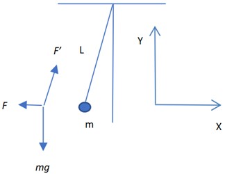
As Fig. 1 shown, to presume the horizontal pulling force is $F$, actually, it equals to the universal gravitation, the gravity of the ball itself is $mg$, the displacement of the ball is $l$, the length of the suspension line is $L$. The pull wire provides a pulling force $F\text{'}$ to the small ball. The resultant force of the ball’s own weight ($mg$) and the universal gravitation ($F$) is equal to $F\text{'}$.

Further, the following formula can be obtained [6-8]. The derivation process of Eq. (1) can be found in Appendix A. The detailed derivation of Eq. (1):

where $F$ the universal gravitation given to the small ball by the steel plate; $mg$ is the ball’s own weight; $l$ is the displacement of the ball; $L$ the length of the suspension line.

The universal gravitation $F$ between the suspended ball and the massive object satisfies the equation [9-12]:

where $G$ is the gravitational constant; $M$ and $m$ are the qualities of steel plates and small ball; $R$ is the distance.

Then:

The above equation does not take the gravity of the rope itself into account. In fact, the rope’s gravity has little effect on the experimental results. We estimate that its impact on the experimental accuracy is less than 1 %.

3. Preparation for experiment

The 30 t steel cube used in the experiment is composed of multiple steel plates of identical specifications, each with a length and width of 1.5 m. When stacked, these steel plates form an overall height of approximately 1.72 m. To facilitate transportation, the steel plates are welded into four separate components. The suspension line is a thin steel wire with a diameter of 0.6 mm, a load-bearing capacity of 45 kg, and a length of 23.2 m. It passes through a pipeline to avoid interference from wind.

Fig. 2 presents a front view of the positions of the steel plate, iron ball, and detector. We would like to point out that this figure is intended to demonstrate that the centers of mass of the small ball and the steel plate, as well as the detector, are at the same horizontal height. It is not designed to quantitatively express the displacement of the ball after attraction. Hence, quantities and units are not labeled.

Fig. 2The front view of the position of the iron plate, ball, and detector

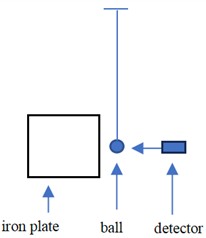
Fig. 3 shows the steel cube and suspended sphere used in the experiment. The high-precision laser displacement detector, which was fixedly installed inside the wall, is not displayed in the figure. This figure was taken by the author Hu Qinggui in July 2023 at the New Campus of Neijiang Normal University, Neijiang, Sichuan, China.

Once the above preparation work is completed, we begin debugging and testing the instruments. During the experiment, the position of the ball was measured 40 times per second. Over a 375-second period, 15,000 sets of measurement data were collected; the average value was then calculated to determine the center position of the oscillating ball.

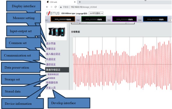
Fig. 4 is a screenshot of the measurement process. We would like to point out that; this figure is a screenshot of the display interface of a high-precision displacement measurement instrument manufactured in Japan. The interface is displayed in Chinese to facilitate use by Chinese users, and we are unable to change Chinese characters to English. The purpose of this figure is to show the operational status of the instrument. The slight blurriness of the image is also due to it being a screenshot, which is inherently less clear than a professionally drawn diagram.

Fig. 3The steel plate and suspended ball in the experiment

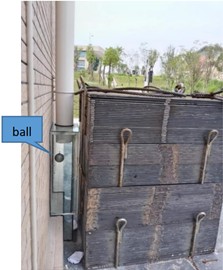
Fig. 4The measurement screenshot

After debugging is finished, we wait for two days to allow the suspension system to stabilize before initiating the experiment. Additionally, the drainage ditch beneath the wall helps reduce the impact of mechanical vibrations. If no drainage ditch is present, a trench should be excavated.

A 30 ton steel plate must be transported to the vicinity of the small iron ball using hoisting equipment, aiming to achieve the gravitational attraction effect on the small ball. Subsequently, the steel plate is moved away to eliminate its gravitational influence on the small ball, and this process is repeated multiple times to obtain replicate experimental data.

During the hoisting operation, the ground vibrations generated primarily include three types: transient impact vibration, low-frequency resonance, and random vibration. These ground vibrations can propagate to the building, causing structural vibrations. Since the suspension wire of the small iron ball is fixed to the building’s roof, building vibrations will induce swaying of the suspension wire – this swaying directly interferes with the stability of the small ball, thereby introducing errors into the experimental results.

To address this issue, a drainage ditch is installed directly beneath the small iron ball. This drainage ditch acts as a vibration isolation barrier, blocking the transmission of ground-induced building vibrations. By mitigating the propagation of vibrations to the suspension system, the adverse impact of vibrations on the experimental results is effectively reduced.

4. Pre-experiment measurement

Based on the experience from the previous experiment, the suspended ball consistently exhibited trembling. To mitigate the impact of this oscillation, 15,000 sets of measurement data were collected in each experimental run, and the average value was calculated to determine the vibration center of the ball.

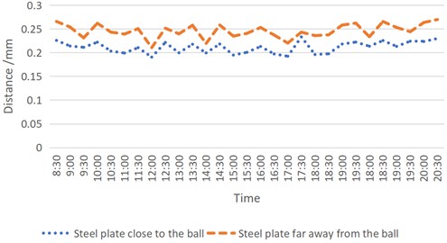
Table 1 presents the average distance values between the ball and the detector on the first day, when the steel cube was positioned close to the ball. From 8:30 to 20:30, measurements were recorded every 30 minutes; each recorded average value was derived from 15,000 individual measurement data points. Fig. 5 is a graph generated based on the data in Table 1.

On the following day, the steel cube was moved far away from the ball. The detector remained fixed inside the wall, with its position unchanged. Table 2 shows the average distance values between the ball and the detector under this condition, and Fig. 6 is a graph constructed from the data in Table 2.

For comparative analysis, Figs. 5-6 were combined to form Fig. 7. As observed in Fig. 7, on the first day (when the steel cube was near the ball), the recorded average distance values were smaller – indicating a greater distance between the ball and the detector. On the second day (when the steel cube was far from the ball), the average distance values were larger, which corresponds to a smaller distance between the ball and the detector. Since all experimental conditions were identical except for the position of the steel cube, it can be inferred that the change in the ball’s position was caused by the gravitational attraction of the steel cube.

To verify the above conclusion, the experiment was repeated on the third and fourth days. Detailed measurement data from these repetitions are not presented here; only the comparative graph (Fig. 8) is provided. As shown in Fig. 8, the results are consistent with those in Fig. 7: larger average distance values were observed when the steel cube was far from the ball, and smaller values were observed when the steel cube was close. This confirms that the change in the ball’s position is indeed attributed by the attraction of the steel cube.

Fig. 5The distance when steel plate is near the ball on the first day

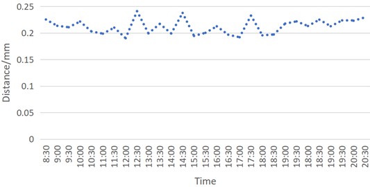
Fig. 6The distance when steel plate is far away from the ball on the second day

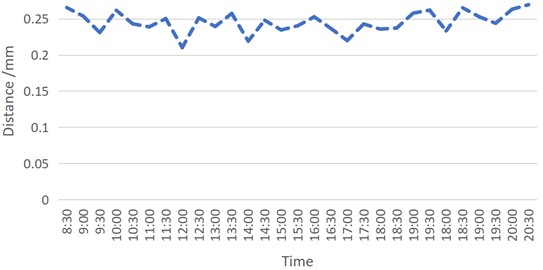
Fig. 7Distance comparison when steel plates is closer and far away from the ball (first and second day)

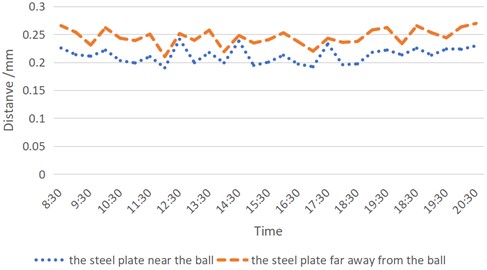
Fig. 8Distance comparison when steel plates is closer and far away from the ball (third and forth day)

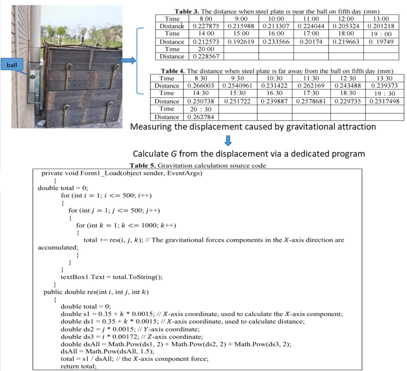
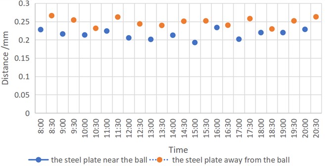
5. The displacement measurement

On the fifth day, we measure the displacement caused by the attraction of the steel plates. At 8:00 in the morning, the steel plate is placed near to attract the ball, 15000 data are collected, and the average value is calculated. Then at 8:30, the steel plate is moved far away from the ball, 15000 data are collected again, and the average value is calculated once more. Just like this, this process is repeated until 20:30.

The statistical results are shown in Table 3 and Table 4. Table 3 displays the measurement values when the steel plate is near the ball. While Table 4 displays the measurement values when the steel plate is far away from the ball. The other environmental factors are same.

Based on Table 3 and Table 4, Fig. 9 is drawn to show the difference. Fig. 9 indicates the attraction of the steel plate leads to the change of the ball’s position.

Fig. 9Distance comparison when steel plates are closer and far away from the ball (fifth day)

From Tables 3 and Table 4, we can see that, at 8:00, the steel plate is placed near the small ball, the distance value is 0.227875 mm. Later, at 8:30, the steel plate was quickly moved far away from the ball, the distance value became 0.256003 mm. Then, the displacement caused by the attraction is S1 = 0.266003 – 0.227875 = 0.038128 mm.

Similarly, at 9:00, the steel plate is placed near the small ball, and the distance value is 0.215988 mm. Later, at 9:30, the steel plate was quickly moved far away from the ball, the distance value became 0.2440961 mm. Then, the displacement caused by the attraction is S2 = 0.2540961 – 0.215988 = 0.0381081 mm.

In this way, we can gain the displacements caused by the attraction as follows:

S3 = 0.231422 – 0.213307 = 0.018115 mm,

S4 = 0.262169 – 0.224044 = 0.038125 mm,

S5 = 0.243488 – 0.205324 = 0.038164 mm,

S6 = 0.239373 – 0.201218 = 0.038155 mm,

S7 = 0.250738 – 0.212573 = 0.038165 mm,

S8 = 0.251722 – 0.192619 = 0.059103 mm,

S9 = 0.239887 – 0.233566 = 0.006321 mm,

S10 = 0.2578681 – 0.20174 = 0.0561281 mm,

S11 = 0.229735 – 0.219663 = 0.010072 mm,

S12 = 0.2517498 – 0.219749 = 0.032008 mm,

S13 = 0.262784 – 0.228567 = 0.034217 mm.

In the next step, we take the average value of S1, S2, S3... S13 as the displacement caused by the attraction.

S = (S1 + S2 + S3 + S4 + S5 + S6 + S7 + S8 + S9 + S10 + S11 + S12 + S13) / 13 = (0.038128 mm + 0.0381081 mm + 0.018115 mm + 0.038125 mm + 0.038164 mm + 0.038155 mm + 0.038165 mm + 0.059103 mm + 0.006321 mm + 0.0561281 mm + 0.010072 mm + 0.032008 mm + 0.034217 mm) / 13 = 0.4448092 mm / 13 = 0.0342161 mm.

The above equation indicates that in this experiment, the displacement caused by the attraction is 0.0342161 mm.

6. The calculation of universal gravitational constant $\mathit{G}$

To facilitate calculations using computer programs, the following mathematical model is established. The large steel cube is treated as an assembly of numerous infinitesimal units, and the gravitational force between the small ball and each of these units is computed.

The small ball is considered a point mass located at the coordinate origin. The $X$-axis passes vertically through the center of the rectangular cube, which has dimensions of 1.5 m in length, 1.5 m in width, and 1.72 m in height. The distance from the rectangular cube to the coordinate origin is 0.35 m; thus, the distance from the cube’s center to the origin is 0.35 + (1.5/2) = 1.10 m.

The mass of the rectangular cube and the small ball are $M$ and $m$ respectively, the gravitational constant is $G$ and the gravitational acceleration is g.

The length, width, and height of the big cube are divided into $n=$1000 parts respectively, then, the big cube is divided into 1000×1000×1000 = 1000000000 tiny cubes. We calculate the gravitational forces between all tiny cubes and the small balls. In this model, the $X$-axis passes through the center of the rectangular cube, the big rectangular cube is divided into four parts in four quadrants. To simplify the calculation, due to symmetry, we only calculate the gravitational forces produced in the first quadrant (Namly, $X>$0, $Y>$0, $Z>$0), at the same time, we only calculate the $X$-axis component of the gravitational force.

For the small tiny cubes in the first quadrant, they are numbered with 1, 2, 3, 4... 1000 along the $X$-axis direction. In the $Y$-axis direction, they are numbered with 1, 2, 3, 4... 500, and in the $Z$-axis direction, they are numbered with 1, 2, 3, 4... 500. For the tiny cube numbered $\left(k,j,i\right)$.

Its $X$-axis coordinate is: 0.35+$k$× 0.0015.

The $Y$-axis coordinate is: $j$×0.0015.

The $Z$-axis coordinate is: $i$×0.00172.

According to the formula of universal gravitation $F=GMm/R^2$, where the parameters $G$, $M$, and $m$ are constants, and the mass of each small tiny cube is $M$/(1000×1000×1000) = $M$/1000000000. For convenience, $G$, $M$/1000000000, and m are not written in the program, and at the same time, we only calculate the $X$-axis component of the gravitational forces.

The program is written in C#; the source code is provided in Table 5.

After the code is executed, its output result is: 160314368.

The above output result means that the total $X$-axis gravitational forces of all the tiny cubes in the first quadrant is:

Then, the total $X$-axis gravitational forces in the four quadrants is:

The above equation means, the gravitation given to the small ball equals to:

We conducted a simple verification for the program in this way: dividing each edge into $n=$2 parts, then, dividing the large rectangular cube into 8 small rectangular cubes. In the next step, we manually calculate the gravitation forces given by the two small rectangular cubes in the first quadrant. The calculation results were compared with those of the computer program ($n$ is set to 2) and they are found to be in consistent agreement. It verifies the rationality of the program.

Afterwards, we set $n=$1000 for program calculation.

In addition, it is worth mentioning that if the large rectangular cube is divided into 100×100×100 = 1000000 parts, the calculation results differ by less than one thousandth only.

Furthermore, in this experiment, if the large rectangular cube is regarded as a whole, in other word, the large rectangular cube is regarded as a mass point. In this case, we calculate the gravitational force, and compare it with the result computed by the computer program to check the extent of the deviation:

The above calculation result indicates when the large rectangular cube is regarded as a mass point, The result is roughly 20 % larger, that is, (0.826 $GMm$-0.65257472 $GMm$)/(0.826 $GMm$) = 20 %. Of course, it is more reasonable to calculate $G$ by dividing the large rectangular cube into one billion small cubes. Here, we just want to find out how big the difference is.

According to the previous introduce, comparing Eq. (3-4), namely $G\frac{Mm}{R^2}=mg\frac{l}{L}$, and $G\frac{Mm}{R^2}=$$0.65257472GMm$.

Therefore:

Then:

It can be rewritten as:

where, $l$ is the displacement caused by the attraction universal gravitation, which is 0.0342161 mm. $M$ is the total mass of the steel plate, the dimensions of the steel plate are 1.5 m, 1.5 m, and 1.72 m, then, the total mass is 1.5 m×1.5 m×1.72 m×7.85×10³ kg/m³ = 30000.3795 kg. $L$ is the length of the line, which is 23.2 m, and $g$ is the gravitational acceleration, it is 9.8 m/s². To substitute data into the Eq. (7):

The above equation shows new $G$ measured in this experiment is 7.3827302×10^-10 N·m²/kg². It has a significant difference with the traditional values. At the same time, it also has a significant difference with our last value gained in July 2021.

Why are our own experimental results different? Although our experiment adopted the same design project, but the experimental environments were different.

1) In 2021, it measured the gravitational constant $G$ between a 2 kg iron ball and a 20 t steel plate. At this time, we measure $G$ between a 5 kg iron ball and a 30 t steel plate.

2) The materials of the suspension lines are different. In 2021, super strong PE fiber was used as the suspension wire. This time, it is steel wire.

3) The measurement environment is different, in 2021, there is a big mountain near the experiment location. This time, there isn’t.

The above are the main differences between two experiments. Perhaps, the reasons lie in those differences. Overall, the second experiment was conducted based on the lessons learned from the first experiment, its result was more reliable.

A novel method is employed herein to measure the gravitational constant $G$ between massive objects, and the results exhibit a significant deviation from traditionally accepted values. From the authors’ perspective, two potential explanations exist for this discrepancy: First, the gravitational constant $G$ itself may not be a true constant, but rather dependent on various factors such as mass, density, and shape. Second, $G$ may indeed be a constant, yet the experimental principle of our approach differs fundamentally from that of the traditional Cavendish torsion balance experiment – this difference in principles could lead to varying measurement results. In short, our current understanding of universal gravitation remains limited.

7. Comparison between our experiment and cavendish torsion experiment

The Cavendish torsion balance experiment is one of the most classic experiments in the history of physics and continues to serve as the most fundamental method for measuring $G$. Its principle is as follows: A balance beam is suspended by a metal wire, with two small balls fixed at each end of the beam. Two larger balls are then used to attract the small balls respectively, causing the balance beam to twist. A reflector is attached to the metal wire to amplify the small torsional angle [13-14].

Compared with the Cavendish torsion balance experiment, our new experimental setup offers greater reliability and smaller systematic errors, for the following reasons:

1) The objects measured in our experiment are significantly more massive – specifically, a 30 ton steel plate and a 5 kg iron ball – whereas the objects in the Cavendish experiment are much smaller. Larger masses help reduce systematic errors.

2) In the Cavendish torsion balance experiment, two large balls are used to attract the two small balls on their respective sides; however, this approach ignores the fact that each large ball also exerts an attractive force on the small ball on the opposite side. This oversight introduces systematic errors.

3) From the perspective of the suspension system, our setup is highly stable, in contrast to the inherent instability of the Cavendish torsion suspension system.

4) Our measuring instrument features digital readout with an accuracy of up to 0.01 microns (10⁻⁸ meters) and can automatically collect 15,000 data points per measurement cycle. By comparison, the Cavendish torsion balance experiment relies on manual observation for data reading, which introduces additional human error.

In summary, the Cavendish experiment imposes extremely stringent requirements on experimental conditions. For instance, uneven temperature distribution can cause thermal expansion or contraction of the metal wire, thereby altering its torsional coefficient. In contrast, our experimental system exhibits greater stability and is subject to fewer error sources [15-16].

8. Discussion on several astronomical and aerospace topics

This project adopts a novel method for measuring the gravitational constant $G$, and the resulting measurement differs significantly from traditional values. In response to this discrepancy, some colleagues may raise the following question: Given the advanced state of modern aerospace technology and the high precision of spacecraft positioning in space, how can this difference be explained?

From the authors’ perspective, modern aerospace technology neither confirms that $G$ is a constant nor verifies that its value is 6.67×10^-11 N·m²·kg^-2. Several examples are provided below for discussion.

1) Navigation Satellite Positioning Systems. The principle of satellite navigation relies on a triangulation-based positioning method, which utilizes high-precision satellite receivers and transmitters. Distances are calculated by receiving and transmitting signals, and this process is primarily related to the Earth’s shape rather than being dependent on $G$.

2) Calculation of Aircraft Landing Positions. Determining an aircraft’s landing position is analogous to solving the problem of predicting where a projectile will land on the Earth’s surface. This result can be computed using the gravitational acceleration $g=$9.8 m/s². Similarly, calculations for spatial landing positioning do not require the value of the gravitational constant $G$.

Verification Based on the Orbits of the Earth and the Moon. Scientists have conducted long-term observational studies on the orbits of celestial bodies, including the Earth, the Moon, and artificial satellites. Some researchers argue that these observational results confirm the validity of the law of universal gravitation and verify the Earth’s mass as 5.97×10²⁴ kg.

However, from the authors’ viewpoint, the Earth’s mass itself is calculated using the formula for universal gravitation. Therefore, such observational results cannot confirm the validity of the law of universal gravitation nor verify that the Earth’s mass is 5.97×10²⁴ kg. In fact, it is the Earth’s mass that determines the orbit of the Moon and the orbits of artificial satellites

In summary, since the Earth’s mass is calculated using a specific value of $G$, subsequent observations (such as those of celestial orbits) cannot be used to verify whether $G$ is equal to 6.67259×10^-11 N·m²/kg² or not.

9. Conclusions

This project employs a 30-ton steel plate to attract a suspended iron ball; by analyzing the displacement changes of the suspended iron ball, the gravitational constant $G$ can be calculated.

The 30 ton steel plate used in the experiment is composed of multiple steel plates with identical specifications, measuring 1.5 meters in length, 1.5 meters in width, and approximately 1.72 meters in height. These steel plates are welded into four separate components to facilitate transportation and handling. The suspension line is made of a thin steel wire with a diameter of 0.6 mm, which can withstand a maximum load of 45 kilograms and has a total length of 23.2 meters. The detector is fixedly mounted on the wall, boasting an accuracy of up to 0.001 mm. It features automatic data collection functionality and a digital display for real-time readings.

During the experiment, the position of the iron ball is measured 40 times per second. Over a duration of 375 seconds, a total of 15,000 measurements are recorded. The average value of these 15,000 data points is calculated to determine the central position of the oscillating iron ball.

Finally, a new value of $G$ is obtained: 7.3827302×10^-10 N·m²/kg. Compared with the traditional Cavendish torsion balance experiment, this new experimental setup exhibits higher stability and reduces the number of error sources.