Numerical study of heat and mass transfer in a relief pipeline with variable diameter

1. Introduction

At present, one of the most important global tasks is to increase energy efficiency, reduce heat and hydraulic losses, and ensure the safety of technological processes. This is especially relevant in industry, energy, and utilities, where liquid transportation systems through closed pipelines are widely used. Reliable and economical operation of such systems requires in-depth scientific analysis. Effective management of these systems largely depends on the correct mathematical modeling of liquid flow processes, taking into account influencing factors such as internal friction, gravitational forces, pipeline geometry, and heat exchange with the environment. Considering such parameters as changes in pipe diameter, inner surface roughness, pipeline inclination angle, and heat transfer with the external environment makes it possible to create models that are close to real operating conditions.

The use of modern numerical modeling software such as COMSOL Multiphysics, ANSYS, MATLAB, and others allows for a detailed analysis of flow and heat transfer processes, preliminary identification of potentially dangerous modes, and the development of safe and energy-efficient operating modes. This is especially important for predicting emergency situations, optimizing control systems, and developing new technological solutions.

A significant contribution to the development of mathematical modeling of gas transportation processes was made by such scientists as I. A. Charny, S. K. Godunov, O. F. Vasiliev, A. F. Voevodin, E. A. Bondarev, M. A. Kanibolotsky, and others. To date, a significant number of scientific studies have been conducted in this area, some of which are briefly discussed below.

The article [1] examines heat exchange on the surface of above-ground pipelines under subzero temperatures. A comparative analysis of the influence of free and forced convection on the temperature of the transported medium is conducted. It was established that in the presence of thermal insulation, forced heat exchange prevails, and the temperature difference between the pipe and the outside air is insignificant. This allows for the use of a simplified boundary condition in the form of temperature equality, which simplifies and increases the accuracy of mathematical modeling of pipeline operation in the cold season.

The paper [2] presents a mathematical model for assessing the thermal properties of pipeline insulation materials. A new type of thermal insulation with a cellular structure filled with air is proposed. Calculations performed using the developed model confirm the high efficiency of such a design for use in heating networks.

By numerically integrating the two-dimensional Navier-Stokes equations in ANSYS Fluent, the flow features at the first resonant frequency were studied [3]. For a pipe with a flange of infinite length and a sharp edge, the effect of piston displacement amplitude on the gas flow rate was analyzed. The phases of gas entry and exit during one oscillation cycle were determined.

The article [4] examines a mathematical model of hydrocarbon gas mixture flow through offshore pipelines on the northern shelf, taking into account real operating conditions. Unlike simplified models, it considers the compressibility and non-ideality of gas, the roughness of pipe walls, the effect of gravity, and complex heat transfer through multilayer walls. An effective numerical solution method is presented, enabling modeling of real flow regimes in complex engineering systems.

In the work [5], an analysis of thermodynamic models of gas flows and a comparison of various mathematical models of gas transportation are carried out. It is shown that excessive simplifications in the model can lead to an incorrect assessment of the thermodynamic characteristics of the flow. Emphasis is placed on the importance of choosing an adequate level of model detail to ensure a reliable prediction of gas transportation system behavior.

The paper [6] describes a quasi-one-dimensional model of steady-state non-isothermal flow of a non-ideal multicomponent gas mixture in ultra-high-pressure offshore gas pipelines. The model takes into account the velocity profile, seabed topography, wall structure, and the possibility of icing. Its effectiveness has been confirmed in calculations for the Shtokman field and the North European Gas Pipeline. Results are partially presented in the book “Models of Sea Gas Pipelines”.

In [7], a generalization of the steady-state flow model to non-stationary processes is presented, including the problem of a gas pipeline transition to a new mode when the intensity of gas extraction changes. It is noted that a significant number of domestic and foreign studies are devoted to modeling gas transportation through main pipelines, which emphasizes the relevance and complexity of this topic.

One of the most universal models and the corresponding numerical algorithms were presented in the monograph by O. F. Vasiliev et al., where the so-called VBVK model is described [8]. This model still serves as the basis for solving a wide range of problems in the field of gas transportation.

In [9], a new stochastic model is proposed to describe the transportation and distribution of gas in gas transportation systems. The model takes into account temperature variation and statistical uncertainty of the parameters of both equipment and the environment. This provides a more accurate description of the actual operating modes of the system.

In [10], a study is conducted on unsteady (transient) flow within a pipeline system. The pressure boundary condition is applied at the inlet, while an air chamber (serving as a damper) with a specified volume is positioned at the outlet. The transmission of a compression shock wave is analyzed using the linearized quasi-one-dimensional approach developed by E. N. Zhukovsky, and the damper behavior is characterized through the I. A. Charny model. To solve the problem, the method of separation of variables is employed. The findings indicate that increasing the volume of the damper leads to a reduction in both the amplitude and frequency of pressure fluctuations due to its damping effect on transient flow behavior.

Despite the large number of scientific studies carried out earlier, the tasks related to the study of processes in pipelines with variable diameters remain relevant. It is especially important to conduct further research to determine the parameters of oil, gas, and heat carrier flows under such conditions and to implement the obtained results in practice. This remains one of the key tasks of modern pipeline transportation.

2. Statement of problems and mathematical model

The problem of determining the state of an elementary relief section of a pipeline is considered, where the law of pressure variation over time is specified at the inlet, and the law of mass flow rate variation of the liquid is specified at the outlet. The boundary condition for the internal energy of the liquid can be imposed either at the inlet or at the outlet of the section.

The initial distributions of velocity, pressure and internal energy of the liquid are given on a linear section of the pipeline, which is defined with its variable diameter $D\left(x\right)$, length $l$, resistance coefficient $\lambda \left(x\right)$, variable leveling height of the pipeline axis $y\left(x\right)$. In this case, the slope of the route of the section is determined as $\sin \alpha =\frac{dy\left(x\right)}{dx}$.

It is necessary to develop a numerical method for solving a stationary problem with a specified mass flow rate of the liquid.

The non-isothermal state of the liquid in a pipeline is described by quasi-one-dimensional equations of conservation of mass, momentum, and internal energy, taking into account local, convective, and other components [11-13]:

Eq. (1):

Here and below $\rho \left(x,t\right)$, $u\left(x,t\right)$, $p\left(x,t\right)$, $T\left(x,t\right)$ – average values of density, velocity, pressure and absolute temperature of liquid in the cross-section $x$at the moment of time $t$ (kg/m³, m/s, Pa, K); $f\left(x\right)=\pi D^2\left(x\right)/4$ – cross-sectional area of the pipeline (m²); $g=$ 9.80665 m/s² – acceleration due to gravity; $\epsilon =c_{B}T$ – internal energy of liquid (J/kg); $c_B=\left(a+bT+c^{\text{'}}{T}^2\right)/\mu$– specific heat capacity of liquid (J/kg/K); $\mu =$ 0.018 kg/mol – molar mass of water; $k_{cp}$ – coefficient of heat transfer from liquid to the environment through the walls of the pipeline and insulation taking into account natural convection [J/(m² sK)]; ${\bar{f}}_{op}\left(x\right)=\pi {\left(D+2\delta \right)}^2/4$ – area of the outer surface of the pipeline, corresponding to 1 linear meter (m); $\delta$ – pipeline thickness (m), $T_{oc}\left(x\right)$ – ambient temperature (K).

The first equation represents the law of conservation of mass: the change in the mass of the liquid in the cross-section of the pipeline occurs due to the difference in the outgoing and incoming liquid flow rates by mass. The second equation represents the law of conservation of momentum: the change in the inertia of the liquid is due to the pressure difference, the friction force (according to the Darcy- Weisbach formula) and the force of gravity. The third equation states that the local and convective transfer of the internal energy of the liquid is due to the dissipation of mechanical energy (in accordance with the quadratic law of resistance) and the heat transfer of the liquid to the environment through the outer surface of the pipeline of unit length.

Let us check the dimensions of the terms of the equation internal energy Eq. (2):

The relationship between pressure and density, given their known characteristic values $p$, $\rho$, is expressed through the modulus of elasticity $k$of the liquid [14-17]:

In particular, for water we can take $p_{*}=$ 101325 Pa, ${\rho }_{*}=$ 998.23 kg/m³ and $k=$2120 MPa, defined for temperature $T_{*}=$293.15 K [14]. Based on this model, in the future the propagation speed of small pressure disturbances is taken according to the dependence $c=\sqrt{k/{\rho }_0}$.

In calculations, the friction resistance coefficient is taken according to the Blasius formula Eq. (3):

A stationary state of rest of the liquid $u\left(x\right)=0$ in the section is considered, or the section operates in a stationary mode with a constant mass flow rate Eq. (4):

3. Method for solving the problem

In this work, Eq. (1) are solved numerically to determine the pressure distribution for an operating pipeline; we turn to the momentum conservation equation in stationary form:

Eq. (5):

Transform Eq. (5) with dependencies:

when $p_{\Delta }=p_{*}-k$ leads to the equation:

Subsequent transformations of the equation yield:

From here we obtain an ordinary differential equation for determining the pressure distribution along the length of a stationary pipeline:

Eq. (6):

To integrate the equation, due to the complexity of its right-hand side, an explicit approximation scheme was used and the values were found $p_{i+1}^0$, where the value of the pressure at the input at the beginning of the process under consideration was used as the boundary condition $p_0^0=p\left(0\right)$.

For $\sin \alpha =\mathrm{c}\mathrm{o}\mathrm{n}\mathrm{s}\mathrm{t}$ and $f=\mathrm{c}\mathrm{o}\mathrm{n}\mathrm{s}\mathrm{t}$an analytical solution of a similar Eq. (6) for a main gas pipeline is given in the work [10]. In addition, under an additional condition, $M^0=0$ the stationary equation of conservation of momentum takes on a simpler form:

which gives a unique barometric pressure distribution in a stationary area according to the volumetric compression of the liquid under the pressure of its upper layers:

Testing the numerical integration method with a step of 1 m for a total section length of 200 m gave a good result. Comparison of the pressure with the results of the above special cases gave a deviation of no more than 0.1 Pa (the relative error does not exceed 10^-6).

With a known initial pressure distribution, $p^0\left(x\right)$ the initial density distribution of the liquid was determined using the formula:

and the speed of the liquid – according to the formula Eq. (8):

Other options for setting the initial conditions are easily adapted to this formulation of the problem based on the initial distribution of mass flow and pressure.

The initial distribution of the internal energy of the transported fluid is determined by solving the stationary equation Eq. (9):

We transform the equation as follows:

Or Eq. (10):

For a given value of the input temperature of the liquid, $T\left(0\right)=T_0^0$ the boundary condition of the equation will be $\epsilon \left(0\right)={\epsilon }_0^0=c_B\left(T_0^0\right)T_0^0/\mu$. In the calculations for water, the formula [17-20] Eq. (11) was used:

In the discretization of the proposed model, an explicit scheme was employed, and the time step was chosen sufficiently small to ensure the stability of the computational process.

To approximate Eq. (10), an explicit scheme was used:

where the values $\lambda$, $D$, $f$, ${\bar{f}}_{op}$, $p^0$ are taken for $i-1$-th node.

The reverse transition to temperature $T_i^0$ is ${\epsilon }_i^0$carried out by solving the cubic equation with respect to temperature $\left(39.02+0.07664T_i^0+1196000/{\left(T_i^0\right)}^2\right)T_i^0-\mu {\epsilon }_i^0=0$.

by dividing the segment in half (the program ensures that the strict condition is met with an accuracy of 10^-10). The resulting value is used for the next node as $T_{i-1}^0$.

The presented numerical method for solving the problem allows for a factor analysis of the stationary process of heat and mass transfer on an elementary relief section with variable internal and external diameters.

The peculiarity of the proposed mathematical model is that it ignores the change in water density depending on temperature. In fact, in the interval 30°-80 °С the absolute change in density is about 2 %, i.e. if we take as the average density of water in this temperature interval 983.2 kg/m³, then the absolute error in the approximation is about 1 %. At the same time, the specific heat capacity of water changes over a large range depending on temperature. Therefore, the internal energy of water was taken with a variable specific heat capacity.

4. Discussion results

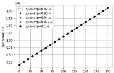
The results obtained below relate to the flow under natural convection conditions, when the flow velocity is sufficiently low than the molasses velocity. According to [20], the quadratic friction resistance regime for which the calculations were performed is characterized by the roughness exit from the thickness of the viscous sublayer. Fig. 1 examines the flow of liquid in a horizontal pipeline ($\mathrm{s}\mathrm{i}\mathrm{n}\alpha$ = 0) with a smooth inner surface, where the roughness coefficient is $k=$0.0001 m. According to [21], new seamless steel and polyethylene pipes have such roughness. In the case of a horizontal pipeline, the main cause of pressure loss is hydraulic resistance caused by friction between the pipe wall and the liquid. As can be seen from the graph, at the smallest pipeline diameter the pressure decreases almost linearly, which indicates a uniform nature of pressure loss along the flow direction. This corresponds to the inversely proportional 5.25th power of the pipe diameter. As the diameter increases, the hydraulic resistance decreases significantly, and the path pressure decrease becomes less pronounced. This explains the tendency to switch to larger diameters of main pipelines.

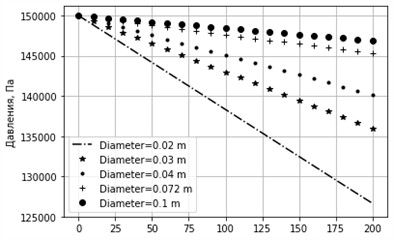
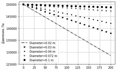
An increase in the roughness coefficient leads to a significant increase in the friction force between the pipe walls and the liquid (Fig. 2). This is especially pronounced in small-diameter pipes; an equivalent roughness of $k=$0.001 m is observed in long-exploited seamless steel and cast-iron pipes [21]. In heavily corroded pipes with significant deposits, the equivalent hydraulicity reaches 0.003 m. With an increase in the pipeline diameter, pressure losses decrease, but compared to the first case, they remain much higher. These data indicate that wall roughness has a significant effect on energy losses in the flow and reduces the overall hydraulic efficiency of the system.

Fig. 1Graph of pressure change for different diameters. sin⁡α= 0, k= 0.0001 m, u= 0.3 m/s

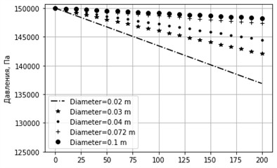
Fig. 2Graph of pressure change for different diameters. sin⁡α= 0, k= 0.001 m, u= 0.3 m/s

According to the proposed model of a real liquid, the path change in pressure is caused by three factors: friction force, gravity force and the local component of the inertial force of the medium transported through the pipeline. The interaction of these three force factors determines the energy mode. As our calculations have shown, in certain intervals of indicators, the role of the third force factor is insignificant, which is explained by an insignificant change in the density of the liquid at a constant mass flow rate of the liquid $\left(f\rho u=\mathrm{c}\mathrm{o}\mathrm{n}\mathrm{s}\mathrm{t}\right)$. Therefore, the main attention is paid to various options for the slope of the route, to the flow rate and the equivalence of the roughness of the pipeline.

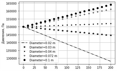
In the results of the calculation of the horizontal pipeline, the factor of gravity is not taken into account and due to the friction force, a practical linear decrease in hydrostatic pressure is observed (Fig. 1 and 2). With a positive slope of the route, $(\sin \alpha >0)$ the force of gravity and the force of friction are directed. Against the flow direction. In this regard, relative to the horizontal route in ascending flows, the loss of pressure increases (Fig. 3 and 4). With an increase in the angle of inclination and equivalent roughness, an increase in the loss of pressure is observed (Fig. 7 and 8). This education is especially noticeable with small pipeline diameters.

With a decrease in the negative slope of the route, the influence of gravity in the formation of the pressure gradient increases and this is expressed by an increase in the pressure gradient. $d{p}^0/dx.$ In this case, the negative pressure gradient can reach zero and positive values $\left(d{p}^0/dx\ge 0\right).$

If the local component of the fluid inertia force and the change in cross-sectional area are ignored, a dependence can be drawn from the equations ${\sin \alpha }_{kp}=-\frac{\lambda }{2D}{u}^2$, that corresponds to the case of compensation of the friction force by the force of gravity.

This case is called a critical slope, after which, with a decrease in the slope, the post-pass flow regime sets in - its energy regime.

The pressure of the post-pass regime can be explained as follows.

In a simple version, $f=\mathrm{c}\mathrm{o}\mathrm{n}\mathrm{s}\mathrm{t}$, $\frac{d\left({\rho }^0{u^0}^2\right)}{dx}\approx 0$ the pressure gradient is determined by the values of the friction force $\frac{\lambda }{2D}\rho u^2$ and the gravitational force $\rho g\sin \alpha$. The friction force acts against the flow direction, and the projection of the gravitational force acts in the direction of the flow. If $\frac{\lambda }{2D}\rho u^2=-\rho g\sin \alpha$ a critical mode is formed, as we discussed above. At, $\frac{\lambda }{2D}\rho u^2<-\rho g\sin \alpha$ part of the energy of the gravitational force compensates for the friction forces. And the excess of the potential energy of gravity is partially twisted to accelerate the flow, and the rest is accumulated in the form of potential energy of compression of the liquid. That is, downstream, an increase in flow is observed.

In Fig. 9-12, the increasing pressure graphs describe the post- saddle flow regime. It follows from the figures that with large pipeline diameters and smaller values of the equivalent roughness, an intensive path increase in pressure occurs. This corresponds to the nature of pipeline transportation of real liquid, since under such conditions the friction force is reduced and is easily compensated by the force of gravity.

When transporting liquid media on descending slopes the post-pass mode is a significant factor that requires the adoption of a decision on the flow rate by creating artificial local resistances. In channels, this is achieved by establishing large irregularities in the flow area. In pipelines, this is achieved by installing throttles, diaphragms and other devices.

In Fig. 13 and 14 the track pressures in the limiting cases of the slope are presented. They show the dominant role of gravity at $\sin \alpha =\text{1}$ (Fig. 13) and at $\sin \alpha =$ –1 (Fig. 14). In other words, with a vertical ascending flow the main energy is spent on overcoming the force of gravity, and with descending flows the role of the friction force in the energy balance is also insignificant. That is, in the limiting slopes of the route the estimate takes place $\rho g\gg \frac{\lambda }{2D}\rho u^2$.

Thus, in the process of designing and calculating inclined pipelines, especially pipelines with large diameters, it is necessary to take into account the possibility of the formation of a post-pass flow and to prevent it. A successful choice of the slope of the pipeline sections allows achieving minimal energy intervention in ensuring forced and free convection in closed and open water heating systems.

Fig. 3Graph of pressure change at different diameters. sin⁡α= 0.001, k= 0.0001 m, u= 0.3 m/s

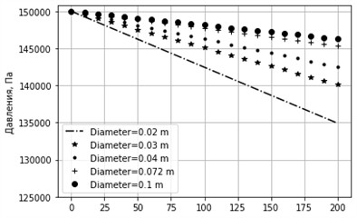
Fig. 4Graph of pressure change for different diameters. sin⁡α= 0.001, k= 0.001 m, u= 0.3 m/s

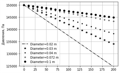
Fig. 5Graph of pressure change at different diameters. sin⁡α= –0.001, k= 0.0001 m, u= 0.3 m/s

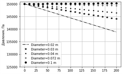
Fig. 6Graph of pressure change for different diameters. sin⁡α= –0.001, k= 0.001 m, u= 0.3 m/s

In Fig. 5 and 6 graphs, cases are considered when the pipeline slope angle is $\sin \alpha =$ –0.001, i.e. downward flows are considered. In this case, the projection of the gravity force coincides with the direction of the liquid flow.

At the same time, the friction force is always directed against the flow. At small negative slopes, the pressure drop along the pipeline is reduced compared to cases without a slope or with a slope against the flow (Fig. 5 and 6). This character of the pressure change is explained by the fact that the potential energy (gravity) of the liquid is converted into kinetic energy. This is confirmed by the Bernoulli equation, which includes the gravitational term. This effect is especially pronounced in pipes with low roughness, where frictional resistance is low. In addition, in large-diameter pipelines, the effect of wall friction is relatively small, and gravitational acceleration has a more pronounced positive influence. Consequently, at small $\sin \alpha <0$ (negative slope angle) pressure loss is reduced, which helps to increase the hydraulic efficiency of the entire system. This can lead to a decrease in the energy consumption of pumping equipment.

Fig. 7Graph of pressure change for different diameters. sin⁡α= 0.01, k= 0.0001 m, u= 0.3 m/s

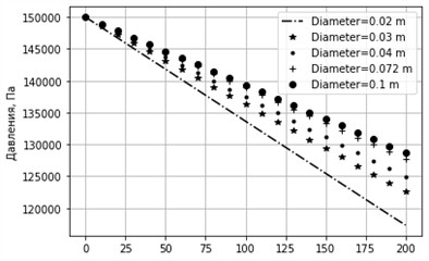
Fig. 8Graph of pressure change for different diameters. sin⁡α= 0.01, k= 0.001 m, u= 0.3 m/s

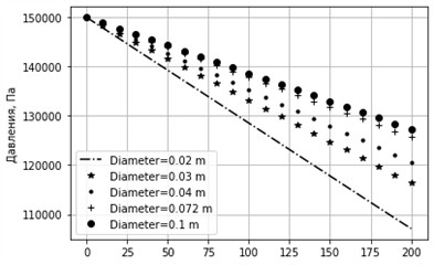
Fig. 9Graph of pressure change for different diameters. sin⁡α= –0.01, k= 0.0001 m, u= 0.3 m/s

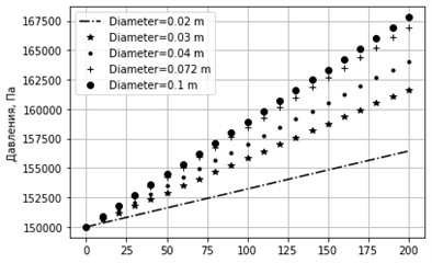
Fig. 10Graph of pressure change for different diameters. sin⁡α= –0.01, k= 0.001 m, u= 0.3 m/s

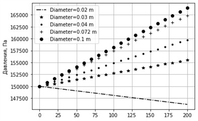
Fig. 11Graph of pressure change for different diameters. sin⁡α= –0.01, k= 0.0001 m, u= 0.4 m/s

Fig. 12Graph of pressure change for different diameters. sin⁡α= –0.01, k= 0.001 m, u= 0.4 m/s

In Fig. 9-12, the cases with a large negative slope of the pipeline are considered, corresponding to the configuration in which the pipe is directed downward in the direction of gravity. Under such conditions, the gravitational component acts in the direction of the flow and contributes to the acceleration of the liquid, which can lead to an increase in pressure along the pipeline or, at the very least, to a noticeable decrease in hydraulic losses. In Fig. 9 and 11, the graphs show that with a large pipe diameter, the pressure along the length can not only be maintained but may even slightly increase. This is explained by the fact that gravitational energy partially compensates for losses due to friction, especially when the pipeline surface is smooth and the flow approaches the laminar regime. However, in Fig. 10 and 12, where the pipe diameter is significantly smaller, the pressure continues to decrease along the length despite the presence of a considerable downward slope. This occurs because, with a small diameter, frictional resistance against the inner pipe walls increases sharply, and all gravitational energy is dissipated to overcome these losses. Thus, the gravitational effect cannot compensate for the increase in specific losses, and the pressure continues to fall. This behavior indicates the existence of a critical relationship between pipe diameter and inclination angle. If the diameter is less than a certain critical value, even a steep inclination cannot provide an increase in pressure due to dominant frictional and turbulence losses. At large negative inclination angles (pipe directed downward), an increase in pressure is possible only at sufficiently large pipe diameters, where gravitational energy prevails over frictional losses. In small-diameter pipes, this effect does not occur, since internal hydraulic losses neutralize the positive contribution of inclination. Therefore, when designing pipeline systems, it is necessary to account for the critical boundary between inclination angle and diameter to ensure optimal conditions for liquid transport with minimal energy costs.

Fig. 13Graph of pressure change for different diameters. sin⁡α= 1, k= 0.0001 m, u= 0.3 m/s

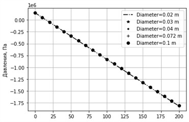
Fig. 14Graph of pressure change for different diameters. sin⁡α= –1, k= 0.0001 m, u= 0.3 m/s

In the process of heat exchange inside the pipeline, the key factors determining the intensity of heat loss of the working medium are the liquid flow rate and the ambient temperature. The obtained results emphasize the importance of a comprehensive analysis of geometric and physical parameters in the design of pipeline systems.

To assess the adequacy of the obtained solution, a comparison was made between the calculation results for a horizontal pipeline and the data obtained on the basis of the experimentally confirmed Darcy-Weisbach formula [25]:

The pressure distribution calculated using the Darcy-Weisbach formula is in good agreement with the results obtained on the basis of the quasi-one-dimensional model.

A linear decrease in pressure along the pipe confirms that the flow is steady and that pressure losses occur mainly due to friction against the pipeline walls.

Fig. 15Comparison of the Darcy-Weisbach model and the quasi-one-dimensional model. u= 0.2 m/s, L= 100 m, μ= 0.001 Pas, Re = ρuD/μ, ρ= 998.23 kg/m3, ε1= 0.0005 m

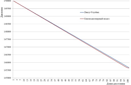
The maximum discrepancy between the two methods is only about 1-2 %, which indicates the high accuracy and practical applicability of the quasi-one-dimensional approach.

Thus, the quasi-one-dimensional model can successfully replace the Darcy-Weisbach method in experimental or simplified calculations, especially under steady-state flow conditions and constant pipeline parameters.

Multiphysics software was used.

Fig. 16Results obtained for the data

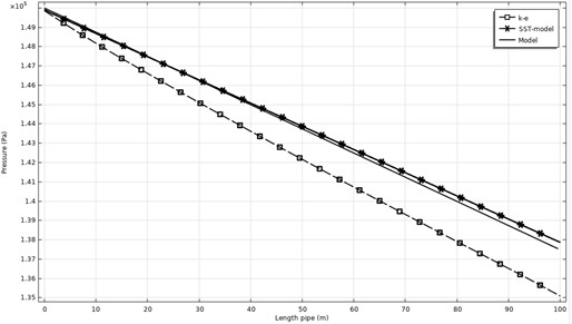
Fig. 16 shows comparative results obtained using the classical $k$-$\epsilon$ model, the Shear Stress Transport (SST) model to describe three-dimensional flows, as well as the new quasi-one-dimensional model proposed by us. The results presented in the graph demonstrate that the calculated curves for the SST model and our model almost completely coincide, indicating a high degree of consistency. Considering that the SST turbulence model provides a more accurate description of transport processes in the presence of solid walls, while the classical $k$-$\epsilon$ model is more suitable for studying jet flows, the outcome of this comparison appears reasonable.

The following feature of the obtained results should be emphasized. In engineering practice, for the calculation of horizontal gas pipelines, an analytical solution to the problem for a quadratic flow regime is used: $p\left(x\right)=\sqrt{{p_{00}}^2-A{M}^{2}x}$.

The features of this solution are analyzed in the works [22, 23]. The pressure traffic is a parabola, the vertex of which is located in the abscissa axis, and the branch extends against the abscissa axis. For a real liquid, obtain results similar to those for an incompressible liquid. That is, the change in flow pressure is practically linear, since at low flow rates, the manifestation of liquid compressibility is insignificant.

In the calculation algorithm we have developed, the value of flow velocity determined during the solution of the problem is used in the process of solving the problem of the path change in the temperature of the liquid in the pipeline. Additional calculations for this problem are carried out by varying the values of the temperature of the liquid at the inlet and the constant temperature of the environment, $T_{oc}$ as well as the values of the generalized heat transfer coefficient in the liquid-wall-environment system and some other data on the object.

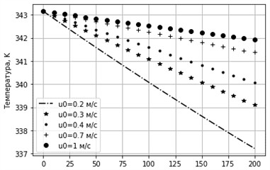
Fig. 16 shows the graphs of the path change in liquid temperature at different values of the internal diameter of the pipeline at $l=$ 200 m, $T_0=$ 343.15 K, $T_{oc}=$ 293.15 K, $\delta =$ 0.00 5m, $K_{sp}=$ 7.5 J/(m² sK). The flow velocity was 0.4 m/s. As shown in the graphs, the liquid temperature decreases almost linearly along the pipeline. For large pipeline diameters, the temperature gradient is insignificant, whereas for small diameters, the intensity of heat transfer increases. This behavior is explained by the fact that with a decrease in the pipeline diameter, the effective heat exchange surface area per unit mass flow rate of liquid increases, which enhances the intensity of heat transfer. Thus, a reduction in the internal diameter of the pipeline leads to an increase in heat transfer intensity, and vice versa. Fig. 18 demonstrates the effect of wall thickness on the path temperature change of the transported liquids. The results were obtained for $D=$ 0.02 m, $K_{sp}=$ 7.5 J/(m² sK) while maintaining the values of the other indicators. According to the graphs, an increase in wall thickness leads to a slower heat transfer. As shown in the work [17] a similar picture of heat exchange in the liquid-pipe-environment system is observed in the absence of flow.

In the technical literature there are scattered data for the heat transfer coefficient $\alpha$ and the average value of the coefficient $K_{sp}.$ In particular, in $\alpha =$ 3500 for the contact of liquid with a solid wall, and in $K_{sp}=$ 1.2 J/(m² sK). For multilayer plane-parallel, cylindrical and spherical bodies, formulas for the generalized heat transfer coefficient are given in [15], which take into account the values of the heat transfer coefficient of multiple layers and the thicknesses and heat transfer coefficients of intermediate layers. In the works [10] it is shown that for the calculation of heat exchangers it is possible to adopt $K_{sp}=$ 7.5 J/(m² sK). Fig. 19 shows the graphs of the path change of the transported medium for different values of the coefficient $K_{sp}$. As expected, with an increase in the value, $K_{sp}$ the intensity of the heat transfer process increases.

Figs. 20 and 21 present the results of the liquid temperature variation under different input and ambient temperature conditions. These results confirm that the intensity of heat transfer increases with a larger temperature difference between the working fluid and the environment.

Let us now proceed to the analysis of temperature changes in the transported liquid as a function of the pipeline parameters.

Fig. 17Change in liquid temperature at different internal diameters. δ= 0.005 m, Ksp= 7.5 J/(m2 sK)

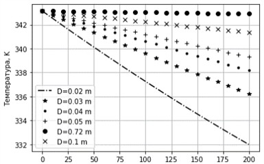
Fig. 18Change in liquid temperature with different pipeline wall thicknesses. D= 0.02 m, Ksp= 7.5 J/(m2 sK)

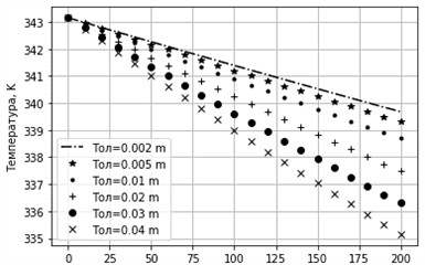
Fig. 19Change in temperature at different values of Ksp. Toc= 293.15 K, δ= 0.005 m, D= 0.05 m

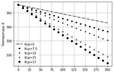
Fig. 20Change in liquid temperature when the inlet temperature changes. Toc= 293.15 K, δ= 0.005 m, D= 0.05 m

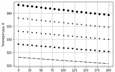
Fig. 21Change in liquid temperature at different ambient temperatures. δ= 0.005 m, D= 0.05 m

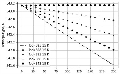
Fig. 22Temperature change with input velocity change. δ= 0.005 m, D= 0.05 m

5. Conclusions

A mathematical model is proposed for steady-state heat and mass transfer processes in a water-based heating system. Under the condition of constant mass flow rate, a quasi-one-dimensional formulation is developed based on the conservation of momentum, taking into account gravitational and frictional forces. An energy equation is derived to describe the variation of the fluid’s internal energy, considering kinetic energy dissipation and heat exchange with the external environment. The resulting nonlinear equations with respect to pressure and temperature are solved numerically using an explicit scheme with sufficiently small time steps. To determine the temperature from the updated internal energy, a cubic equation is formulated and solved using the bisection method.

In this study, the hydraulic and thermal characteristics of fluid transport in closed pipelines were analyzed under various conditions, including variations in pipe diameter, internal surface roughness, inclination angle, thermal conductivity of the pipe material, and ambient temperature. Graphical analysis showed that the greatest influence on pressure and temperature losses is exerted by pipe diameter, flow velocity, gravity, and the temperature difference between the liquid and the surrounding environment. Minimal pressure losses were observed in smooth, horizontal pipes of large diameter, whereas increased roughness, small diameters, and inclined sections led to significantly higher losses.

In the heat transfer analysis, it was found that the thermal conductivity of the pipe material and the ambient temperature are key parameters. Higher thermal conductivity and flow rate lead to more intense heat exchange and, consequently, greater heat loss. The modeling performed in the COMSOL Multiphysics environment demonstrated a high degree of agreement between the results of the proposed model and the SST turbulence model, which confirms the adequacy of the developed approach in describing complex turbulent flows.

Thus, the obtained results enable more accurate modeling of fluid motion in pipeline systems and can be applied in the development of effective energy-saving solutions, optimization of technological processes, and ensuring reliable operation of heat supply, water distribution, and industrial liquid transport systems.

In this study, a comprehensive analysis of hydraulic and thermal processes in closed pipelines was carried out, and a new quasi-one-dimensional mathematical model was proposed. The developed model is based on the conservation equations of mass, momentum, and internal energy, while taking into account gravitational forces, frictional resistance, and heat exchange with the external environment. In the model, kinetic energy dissipation and heat transfer effects are explicitly included.

The research results demonstrated that pipe diameter, flow velocity, inclination angle, and ambient temperature are the most influential parameters affecting fluid motion and heat losses. Furthermore, the results obtained in COMSOL Multiphysics were compared with the SST model and showed a high degree of consistency, which confirms the reliability and adequacy of the proposed model.

Thus, the developed model makes it possible to more accurately simulate heat and mass transfer processes in closed pipeline systems and can be effectively applied for the development of energy-saving technologies, optimization of heat and water supply systems, and improvement of industrial liquid transportation efficiency.