Short-term electricity load interval estimation algorithm based on OS-ELM feature enhancement for SVR

Wei, Yaxing; Han, Jiamao; Zhao, Bin; Chen, Yujia; Ao, Wei; Ma, Mingzuo; Man, Lai

doi:10.21595/jme.2026.25355

Journal of Measurements in Engineering

Browse Journal

Submit article

Published: September 27, 2026

Check for updates

Short-term electricity load interval estimation algorithm based on OS-ELM feature enhancement for SVR

Yaxing Wei¹

Jiamao Han²

Bin Zhao³

Yujia Chen⁴

Wei Ao⁵

Mingzuo Ma⁶

Lai Man⁷

¹Chongqing University, School of Big Data and Software Engineering, Chongqing, 400000, China

^{2, 3, 4, 5, 6, 7}Inner Mongolia Power Group Inner Mongolia Electric Power Digital Research Company, Hohhot, 010000, China

Corresponding Author:

Yaxing Wei

Cite the article Download PDF

Article in Press

Downloads 0

Abstract

Short-term power load forecasting is crucial for power system dispatch and market transactions. However, the dynamic, nonlinear, and uncertain nature of loads poses challenges for accurate interval estimation. This paper proposes a short-term load interval estimation algorithm based on online sequence extreme learning machine (OS-ELM) feature enhancement and support vector regression (SVR). Rather than a simple model stacking approach, it constructs a dynamically collaborative two-stage prediction architecture: OS-ELM serves as a real-time feature generator, adaptively capturing concept drift in data streams to produce dynamically enhanced features; these features are then fed into an SVR model for high-precision point prediction. Finally, dynamic confidence intervals are constructed based on the empirically updated prediction error distribution. Experiments validate the approach using actual summer data (26,304 samples) from a provincial power grid in China. Results demonstrate outstanding point prediction performance with an RMSE of 236.7 MW and MAPE of 1.80 %, outperforming benchmark models including SARIMA, LightGBM, LSTM, and Transformer. For interval forecasting, at a 95 % confidence level, it achieves 94.5 % interval coverage with an average interval width of 148.7 MW, striking a good balance between coverage and precision while maintaining high interval calibration quality. Furthermore, the scheduling scheme based on this algorithm strictly controls system voltage fluctuations within ±0.4 p.u., significantly enhancing system operational stability. This algorithm provides a solution for short-term load forecasting that combines high accuracy, strong adaptability, efficient computation, and reliable uncertainty quantification capabilities.

Short-term electricity load interval estimation algorithm based on OS-ELM feature enhancement for SVR

Highlights

A dynamically collaborative two-stage architecture uses OS-ELM as a real-time feature generator to capture concept drift, feeding enhanced features into SVR for accurate point prediction.
High accuracy and reliable intervals: RMSE of 236.7 MW and MAPE of 1.80% outperform SARIMA, LightGBM, LSTM, and Transformer; 94.5% coverage at 95% confidence with a 148.7 MW average width.
Improved operational stability: the scheduling scheme keeps voltage fluctuations within ±0.4 p.u., combining accuracy, adaptability, efficiency, and reliable uncertainty quantification.

1. Introduction

Load forecasting is a well-established research topic in power systems. It involves analyzing historical data [1] based on known power system conditions, economic factors, social influences, and meteorological data to uncover intrinsic relationships and development patterns, enabling preliminary estimations and predictions of load trends. Traditional load forecasting methods have limitations when dealing with massive high-dimensional data, dynamic environmental changes, and nonlinear characteristics [2]. The Online Sequential Limit Support Vector Regression (OS ELM Features + SVR) offers a novel solution for short-term load interval estimation through its dynamic adaptability and computational efficiency. Short-term power load forecasting is a core component of power system dispatch, generation planning, and market transactions, where its accuracy directly affects grid operational efficiency and economic performance [3]. Support vector regression demonstrates excellent generalization performance in small-sample and high-dimensional data scenarios based on the principle of minimizing structural risk, but its static model is difficult to adapt to real-time data updates [4]. OS ELM Feature + SVR extends Support Vector Regression to dynamic environments through an Online Sequential learning mechanism, enabling real-time updates to prediction models to effectively handle changes in data streams. Applying this algorithm to power load forecasting can significantly reduce computational costs and enhance prediction timeliness [5], thereby providing reliable support for power system optimization and scheduling.

Behmiri et al. applied time series regression and neural networks to power load forecasting [6]. Time series regression models utilized historical data and mathematical formulations to describe the relationship between temperature and power load, providing an intuitive measure of temperature's influence. Neural networks could process and learn the nonlinear temperature-load relationships, capturing more complex patterns and interactions. The network structure and parameters were automatically adjusted based on input data characteristics to accommodate different distributions and prediction tasks. However, time series regression models typically assumed linear temperature-load relationships, whereas real-world scenarios exhibit nonlinearity, limiting prediction accuracy. Kalhori et al. developed a data-driven knowledge-based system for long-term regional load prediction under uncertain evidence [7]. This algorithm could fully utilize historical load data and other relevant data for learning and reasoning, adapting to regional and temporal load characteristics. By continuously learning and updating data, the model could automatically adjust prediction results. Real-world predictions often involved uncertain evidence like missing, inaccurate, or conflicting data. The algorithm enhanced robustness by handling such uncertainty through probabilistic and fuzzy reasoning. Its inference mechanism derived future load trends from current data and existing knowledge, supporting decision-making. However, its performance heavily depended on data quality – excessive noise, missing values, or outliers significantly impair learning and inference capabilities. Chauhan et al. employed Support Vector Machines (SVMs) for short-term power load forecasting [8]. SVMs optimized the objective function through margin maximization, enabling them to capture nonlinear data relationships. This made them particularly suitable for complex scenarios where power load interacted with multiple factors like weather conditions and holiday effects. By utilizing kernel functions to project data into high-dimensional feature spaces, SVMs circumvented the restrictive distributional assumptions inherent in traditional methods. Even with limited training samples, SVMs could deliver robust predictions by relying on support vectors, thus mitigating overfitting risks. However, this approach demanded substantial feature engineering efforts, necessitating manual extraction of daily and weekly cyclical load patterns. The model's performance degraded considerably when key predictive features were omitted. Bayram et al. employed an LSTM network integrated with a dynamic drift adaptive learning framework for interval load forecasting [9]. The LSTM architecture effectively captured both long-term and short-term temporal dependencies through its gating mechanism, enabling adaptation to power load periodicity and trend characteristics, which made it particularly suitable for analyzing non-stationary time series data. Through real-time parameter updates and structural adjustments to the network, the model demonstrated enhanced capability to accommodate sudden load pattern variations. The dynamic drift adaptation mechanism facilitated automatic model refinement, significantly reducing dependence on expert intervention or manual parameter calibration, consequently lowering operational expenditures. However, LSTM's network structure, learning rate, and other hyperparameters significantly affected performance, and the dynamic drift mechanism required additional adjustments to update frequency and amplitude, making the tuning process time-consuming and dependent on experience. If the update frequency was too high, the model may oscillate due to data noise; if too low, it could not adapt to changes in a timely manner. LSTM tended to fail when handling ultra-long-term dependencies, and the dynamic drift mechanism may sacrifice generalization ability due to overfitting recent data, especially when the data distribution changes abruptly.

The core innovation of this work lies not in simple model stacking, but in constructing a two-stage collaborative prediction architecture with explicit temporal adaptability. Its uniqueness and advantages over existing methods are demonstrated as follows:

Compared to single Online Sequential Extreme Learning Machine (OS-ELM): While OS-ELM efficiently processes data streams, its capability to fit complex nonlinear load dynamics through a linear output layer is inherently limited as a single-hidden-layer network, and it remains sensitive to outliers. This paper innovatively repositioned OS-ELM as a dynamic feature generator. Its core function is to adapt in real-time to data distribution drift, providing time-varying, robust high-dimensional feature representations for the more powerful nonlinear regressor in the backend. This combines OS-ELM's online learning efficiency with SVR's strong nonlinear modeling capability and structural risk minimization advantage, achieving synergistic improvement in prediction performance.

Compared to traditional static ELM+SVR stacked models: Conventional static feature stacking models fix the feature extraction layer post-training, failing to adapt to time-varying load patterns. The key innovation of this framework lies in introducing an “online feature sequence evolution” mechanism. Through OS-ELM's recursive weight updates, the model's feature space dynamically adjusts with new data batches, ensuring features fed to SVR consistently capture the latest data patterns. This transforms the entire model from a “static fitter” to a “dynamic adaptive system,” significantly enhancing its modeling capability for non-stationary time series.

Compared to deep benchmark models like LSTM and Transformer: Deep models possess powerful representation capabilities but typically come with challenges such as high computational cost, hyperparameter sensitivity, and complex online update strategies. This framework offers a lightweight, efficient, and more interpretable technical path. By leveraging OS-ELM's analytical solution properties and SVR's convex optimization, it avoids iterative gradient training inherent to deep learning. Through clear dynamic feature updates and periodic SVR batch retraining, it provides a stable, efficient online learning solution. Combined with dynamic error distribution estimation, it delivers reliable interval predictions without complex probabilistic modeling.

2. Short-term electricity load interval estimation algorithm

2.1. Short-term electricity load enhanced feature set construction based on extreme learning machines

Historical short-term power load data is collected as input for the Extreme Learning Machine (ELM), which generates intermediate load predictions. The hidden layer outputs of the ELM are extracted as additional features and concatenated with original load features, including weather conditions and temporal information [10], to construct an enhanced feature set for short-term load estimation. This augmented feature set serves as input to the subsequent support vector regression algorithm. The Extreme Learning Machine (ELM) is a single-hidden-layer feedforward neural network (SLFN) known for its fast learning speed. In ELM, the input weights and biases of the hidden layer are randomly assigned and fixed [11], and the output weights are analytically determined by minimizing the training error. Given $N$ short-term power load training datasets ${(x_{i}, o_{i})}_{i = 1}^{N}$ , where $x_{i} = [x_{i 1}, x_{i 2}, \dots, x_{i n}]$ is the input historical power load vector and $o_{i}$ is the corresponding expected power load output value. The mathematical model of the extreme learning machine with $\tilde{N}$ hidden layers and an activation function of $σ (x)$ can be expressed as:

1

\sum_{i = 1}^{\tilde{N}} β_{i} σ (w_{i} \cdot x_{j} + b_{i}) = o_{j},

where, $j = 1,2, \dots, N$ , $w_{i} = [w_{i 1}, w_{i 1}, \dots, w_{i n}]^{T}$ is the weight connecting the $i$ -th hidden layer neuron and the input layer, $b_{i} = [b_{i 1}, b_{i 2}, \dots, b_{i \tilde{N}}]^{T}$ is the bias of the $i$ -th hidden node, and $β_{i} = [β_{i 1}, β_{i 2}, \dots, β_{i n}]^{T}$ is the weight connecting the $i$ -th hidden layer neurons and the output layer.

Eq. (1) can be simplified in matrix form as follows:

2

H β = O .

In Eq. (2), the expression of matrix $H$ is as follows:

3

H (w_{1}, \dots, w_{\tilde{N}}, x_{1}, \dots, x_{N}, b_{1}, \dots, b_{\tilde{N}}) = {[\begin{matrix} σ (w_{1} \cdot x_{1} + b_{1}) & \dots & σ (w_{\tilde{N}} \cdot x_{1} + b_{\tilde{N}}) \\ ⋮ & \dots & ⋮ \\ σ (w_{1} \cdot x_{N} + b_{1}) & \dots & σ (w_{\tilde{N}} \cdot x_{N} + b_{\tilde{N}}) \end{matrix}]}_{N \times \tilde{N}},

where, $H$ is the hidden layer output matrix.

By solving for the output weights [12], the expression that guarantees the minimum value of the loss function is as follows:

4

\min_{β} ‖Hβ - O‖ .

By solving the least squares solution of Eq. (4), the expression that guarantees the minimum of the loss function is as follows:

5

‖ Hβ - O ‖ = ‖ H H^{†} O - O ‖ = \underset{β}{m i n} ‖H β - O‖,

where, $H^{†}$ $H^{†}$ is the Moore-Penrose generalized inverse of the hidden layer output matrix $H$ .

Extreme Learning Machines lack robustness against outliers in power load data. Introducing a regularization coefficient balances training error and output weights in power load forecasting [13]. Leveraging the sparse property of the L1 norm, the loss function in Eq. (4) is modified to the following objective function:

6

\{\begin{array}{l} \min_{β} {‖e‖}_{1} + \frac{1}{γ} {‖β‖}_{2}^{2}, \\ O - H β = e, \end{array}

where, $γ >$ 0 is the regularization coefficient, used to balance training error and output weight sparsity; ${‖‖}_{1}$ denotes the L1 norm. To solve this non-smooth optimization problem involving the L1 norm, an augmented Lagrangian function is employed to introduce the auxiliary variable $z$ , reformulating the problem into an equivalent constrained form:

7

\underset{β, z}{m i n} \frac{1}{2} |H β - T |_{2}^{2} + λ| z |_{1} s.t. H β - z = 0 .

The corresponding augmented Lagrangian function is:

8

Q_{ρ} (β, z, η) = \frac{1}{2} ‖ H β - T ‖_{2}^{2} + λ ‖ z ‖_{1} + η (H β - z) + \frac{ρ}{2} ‖ H β - z ‖_{2}^{2},

where, $η \in R^{m}$ is the Lagrange multiplier. $ρ >$ 0 is the penalty parameter.

Using the alternating direction method of multipliers for iterative solution, the recursive function at iteration $k + 1$ is obtained as follows:

9

\{\begin{array}{l} β_{k + 1} = a g r m i n_{β} Q_{ρ} (β_{k}, z_{k}, η_{k}), \\ z_{k + 1} = a g r m i n_{β} Q_{ρ} (β_{k}, z_{k}, η_{k}), \\ η_{k + 1} = η_{k} ς (H β_{k + 1} - T_{k + 1}) . \end{array}

The convergence condition is that both the original residuals and dual residuals are less than the preset tolerance.

The L1 norm leverages its sparsity properties to mitigate outlier interference. By incorporating the training error $e$ , the output layer weights $β$ are adaptively updated through error feedback, establishing a robust power load prediction model resistant to outliers. Through this process, intermediate load predictions are generated, where the hidden layer outputs from the extreme learning machine serve as features. These are then combined with other support vector machine input features to construct an enhanced feature set for short-term power load estimation.

2.2. Short-term power load regression prediction model based on support vector regression

Historical load data is integrated with temporal features (including hour of day, day of week, and holiday indicators), meteorological parameters (such as temperature, humidity, wind speed, and precipitation), economic factors (particularly electricity prices), and the hidden layer outputs from the extreme learning machine to form an enhanced feature set for short-term load forecasting. This comprehensive feature set serves as input to the support vector regression model, enabling construction of an accurate short-term load prediction framework. The support vector regression algorithm demonstrates exceptional capability in approximating nonlinear functions with arbitrary precision while guaranteeing global optimal solutions [15]. Known for its rapid convergence, this algorithm has been widely adopted for time series regression tasks. It excels particularly in handling small-sample, nonlinear, and high-dimensional pattern recognition problems, with successful extensions to function approximation and other regression applications [16]. The fundamental principle of applying support vector regression to short-term load forecasting involves identifying the optimal separating hyperplane under linear separability assumptions, as described below:

10

w^{T} \times x \times b = 0,

where, $x$ is the power load input vector, $w$ is the weight coefficient, and $b$ is the bias.

The short-term power load forecasting problem is a linear inseparable problem. Therefore, kernel functions are introduced to map the power load input vector from a low-dimensional space to a high-dimensional space, where a separating hyperplane is sought [17]. This allows some sample points to be free, i.e., slack variables are introduced, and a soft-margin separating hyperplane is constructed. The support vector machine-based short-term power load regression forecasting model is constructed as follows:

11

\{\begin{array}{l} \underset{w, b}{m i n} \frac{1}{2} {‖W‖}^{2} + ς \sum_{i = 1}^{m} ξ_{i}, \\ s . t . y_{i} (w^{T} φ (x_{i}) + b) \geq 1 - ξ_{i}, \end{array}

where, $ς$ $?$ $ς$ is the penalty coefficient, $f (x^{(i)})$ $φ (x^{(i)})$ $φ (x^{(i)})$ is the mapping function to the high-dimensional feature space, and $ξ_{i}$ $?_{i}$ $ξ_{i}$ is the slack variable.

Short-term power load forecasting is a quadratic convex optimization problem [18], and the corresponding Lagrangian function is constructed as follows:

12

Q (w, b, ξ, α) = \frac{1}{2} w^{T} w + ς \sum_{i = 1}^{m} ξ_{i} - \sum_{i = 1}^{m} α_{i} [y_{i} (x^{T} + b) - 1 + ξ_{i}],

where, $α$ represents the Lagrange multiplier.

By organizing and substituting, we obtain the dual optimization problem for short-term power load forecasting:

13

\{\begin{matrix} \max_{α} W (α) = \sum_{i = 1}^{m} α_{i} - \frac{1}{2} \sum_{i, j = 1}^{m} x_{i} y_{i} α_{i} α_{j} ⟨φ (x_{i}), φ (x_{j})⟩, \\ s . t . \sum_{i = 1}^{m} α_{i} y_{i} = 0 . \end{matrix}

The expression for the support vector machine regression function in final short-term power load forecasting is as follows:

14

f (x) = \sum_{i = 1}^{n} α_{i} y_{i} ⟨φ (x), φ (x_{i})⟩ + b .

The expression for the inner product kernel defined by Mercer’s theorem is as follows:

15

K (x_{i}, x_{j}) = ⟨φ (x_{i}), φ (x_{j})⟩ .

The final power load forecasting model of the support vector machine is as follows:

16

f (x) = \sum_{i = 1}^{n} α_{i} y^{(i)} K (x, x_{i}) + b .

Using Eq. (16), we obtain the regression prediction value of short-term power load data $x$ .

2.3. Online sequential limit support vector regression algorithm for short-term power load prediction

To extend the capability of the support vector regression algorithm to process dynamically incoming data, an online sequential extreme support vector regression algorithm is developed. Although OS-ELM possesses efficient online learning capabilities, its random initialization and reliance solely on fitting through a linear output layer impose limitations on the model’s expressiveness and robustness when handling complex nonlinear dynamics of power loads. In this framework, OS-ELM’s hidden layer parameters remain fixed after initialization, adhering to standard ELM/OS-ELM design principles. Its “online sequence” property manifests in the recursive update of output weights, enabling the hidden layer's output features to adapt to dynamic shifts in data distribution. This design preserves ELM's computational efficiency while endowing the model with adaptability to concept drift through its feature evolution mechanism.

Assuming the initial data sample of the power load database is $Z_{0} = {(x_{i}, y_{i}) | x_{i} \in R^{m}}_{i = 1}^{N_{0}}$ , the optimization problem for short-term power load forecasting is equivalent to minimizing the $‖ H_{0} W_{0} - Y_{0} ‖$ problem [19], and the output matrix of the hidden layer weights $W_{0}$ is calculated:

17

W_{0} = (G + H_{0}^{T} H_{0})^{- 1} H_{0}^{T} Y_{0},

where, $G$ represents the regularization factor.

To simplify the representation, let $A_{0} = G + H_{0}^{T} H_{0}$ , $B_{0} = H_{0}^{T} Y_{0}$ , where $H_{0}$ is the hidden layer feature mapping matrix, which can output the vector $Y_{0}$ :

18

H_{0} = [\begin{matrix} σ (w_{1}, x_{1}) & \dots & σ (w_{L}, x_{1}) & 1 \\ ⋮ & ⋮ & ⋮ & ⋮ \\ σ (w_{1}, x_{N_{0}}) & \dots & σ (w_{L}, x_{N_{0}}) & 1 \end{matrix}],

19

Y_{0} = [y_{1}, y_{2}, \dots, y_{N_{0}}]^{T},

where, $σ$ represents the activation function.

The equivalent form of Eq. (18) is shown as follows:

20

W_{0} = A_{0}^{- 1} B_{0} .

At this time, the newly added online load sequence updates enter the power system [20]. It is assumed that the flow of the newly added power load online sequential is $Z_{1} = {(x_{i}, y_{i}) | x_{i} \in R^{m}}_{i = N_{0} + 1}^{N_{0} + N_{1}}$ , where $N_{1}$ represents the number of data points in the power load sequence flow $Z_{1}$ $Z_{1}$ . The optimization problem corresponding to the short-term power load forecasting is expressed as:

21

\min \{‖[\begin{matrix} H_{0} \\ H_{1} \end{matrix}] W_{1} - [\begin{matrix} Y_{0} \\ Y_{1} \end{matrix}]‖\},

where:

22

H_{1} = {[\begin{matrix} σ (w_{1}, x_{N_{0} + 1}) & \dots & σ (w_{L}, x_{N_{0} + 1}) & 1 \\ ⋮ & ⋮ & ⋮ & ⋮ \\ σ (w_{1}, x_{N_{0} + N_{1}}) & \dots & σ (w_{L}, x_{N_{0} + N_{1}}) & 1 \end{matrix}]}_{N_{1} \times (L + 1)},

23

Y_{1} = [y_{N_{0} + 1}, y_{N_{0} + 2}, \dots, y_{N_{0} + N_{1}}]^{T} .

The calculation process of the hidden layer weight output matrix $W_{1}$ $W_{1}$ $W_{1}$ is as follows:

24

W_{1} = (A_{0} + H_{1}^{T} H_{1})^{- 1} {[\begin{matrix} H_{0} \\ H_{1} \end{matrix}]}^{T} [\begin{matrix} Y_{0} \\ Y_{1} \end{matrix}] .

Let $A_{1} = A_{0} + H_{1}^{T} H_{1}$ , the calculation of $A_{1} = A_{0} + H_{1}^{T} H_{1}$ in Eq. (24) is as follows:

25

{[\begin{matrix} H_{0} \\ H_{1} \end{matrix}]}^{T} [\begin{matrix} Y_{0} \\ Y_{1} \end{matrix}] = (A_{1} - H_{1}^{T} H_{1}) W_{0} + H_{1}^{T} Y_{1} .

Based on the above content, the update formula for the hidden layer output weight $W_{1}$ $W_{1}$ is as follows:

26

W_{1} = W_{0} + A_{1}^{- 1} H_{1}^{T} (Y_{1} - H_{1} W_{0}) .

When the $k + 1$ batch of online sequential $Z_{k + 1}$ reaches the power system, the corresponding expression for the hidden layer weight output matrix is as follows:

27

W_{k + 1} = W_{k} + A_{K + 1}^{- 1} H_{K + 1}^{T} (Y_{k + 1} - H_{k + 1} W_{k}) .

Through the aforementioned process, the short-term power load forecasting values are generated by processing the input online load sequence using a combined approach of extreme learning machines and support vector regression algorithms.

The online learning process of this framework can be clearly divided into two parallel levels:

High frequency dynamic feature update layer (OS-ELM): For each newly arrived data block, OS-ELM immediately updates its output weight $β$ through recursive least squares (Eqs. (27-28)), thereby generating real-time dynamic hidden layer features that reflect the latest data distribution. This process is block by block, online, and real-time.

Low frequency global model update layer (SVR): The SVR model is not updated with each data block. The system sets an update cycle (e.g. every 24 hours or whenever accumulated data reaches a predetermined scale). When an update is triggered, the system will combine all accumulated historical samples to form a new training set and conduct a complete retraining of the SVR model. After training, the SVR model will be used for all subsequent predictions until the next update cycle.

The advantage of this collaborative mechanism of “OS-ELM dynamic feature flow+SVR periodic retraining” is that OS-ELM ensures real-time adaptability of feature representation to concept drift with extremely low computational cost; The periodic retraining of SVR ensures the optimal global nonlinear fitting ability of the model while avoiding complex online kernel function optimization problems. The update frequency of SVR is an adjustable hyperparameter that strikes a balance between model adaptability and computational overhead.

2.4. Short-term power load interval estimation algorithm based on confidence intervals

Based on the short-term power load forecasting results, the power system's load interval is estimated. Section 2.3 outputs the confidence interval of forecasted loads at specified confidence levels, determining the probability that this interval contains the actual load value. Historical data and forecasting results serve as analysis samples, with load forecasting error defined as the difference between actual load $L_{a}$ and forecasted load $L_{b}$ at any given time:

28

e = \frac{L_{b} - L_{a}}{L_{a}} .

Daily load sampling collects 24 hourly measurements. Given significant variations in relative error fluctuations across different time intervals and load levels, historical load samples require stratified interval grouping for relative error statistical analysis. Initial stratification divides time intervals into valley, peak, and off-peak segments based on typical daily load patterns. Subsequent merging combines adjacent low-frequency segments until each merged zone meets minimum sample size requirements. The nonlinear characteristics of power load curves cause forecasting errors to exhibit non-Gaussian, skewed distributions. By applying relative errors $e_{i}$ into Eq. (28), we obtain the distribution function for any relative error $e$ . The load value confidence interval is then determined at specified confidence level $υ (0 < υ < 1)$ , where any load value $L$ satisfies:

29

P ({\hat{L}}_{m i n} < L < {\hat{L}}_{m a x}) = 1 - υ .

The interval $({\hat{L}}_{m i n}, {\hat{L}}_{m a x})$ is called the confidence interval at the confidence level of $L$ . This means that the probability of the random interval $({\hat{L}}_{m i n}, {\hat{L}}_{m a x})$ containing the actual load value is $1 - υ$ . In this paper, when estimating the power load interval, a symmetric probability interval is taken, that is, $υ_{1} = υ / 2$ and $υ_{2} = 1 - υ / 2$ .

For short-term power load interval estimation, the online sequential extreme learning machine generates 24-hour ahead load predictions for the power system. Test samples are analyzed to derive statistical characteristics of historical forecasting errors, enabling subsequent interval partitioning. For each predicted load value, its corresponding historical load interval is identified, and the associated relative error partition interval is determined. The cumulative probability distribution function is obtained through integration, identifying the $υ / 2$ and $1 - υ / 2$ points of the load value, obtaining the confidence interval for that load forecast value, and outputting the short-term power load interval estimation results.

3. Experimental analysis

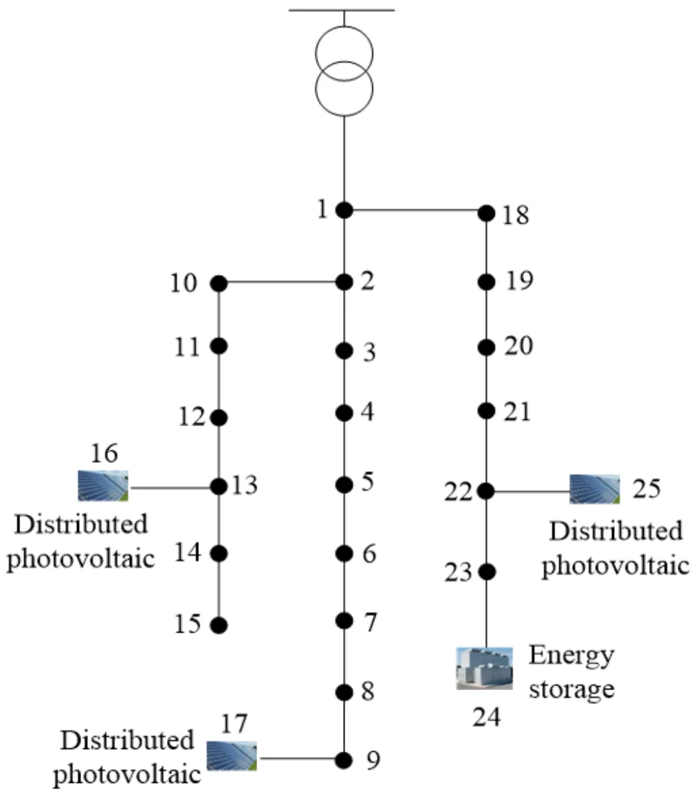
The studied algorithm is applied to a distributed power system with 25 IEEE nodes, which incorporates photovoltaic distributed power sources. Its topology diagram is shown in Fig. 1.

The equipment parameters of the power system are shown in Table 1.

Fig. 1Topology diagram of power system.

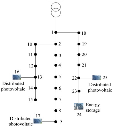
Table 1Parameters of power system equipment

Category	Parameter	Parameter units	Value
Generator	Rated power	MW	500
	Active power regulation range	MW	100-500
	Governor response time	s	2.5
Transformer	Rated capacity	MVA	100
	Percentage of short-circuit impedance	%	0.1
	No-load loss	kW	20
Transmission line	Wire model	–	LGJ-400/50
	Line length	km	15
	Charging capacitor	μF/km	0.012
Distributed photovoltaic	Installed capacity	MW	10
Energy storage	Energy storage capacity	MWh	50
	Charging power	MW	3
	Discharge power	MW	2
Time of use electricity price during peak hours		Yuan / kWh	0.85

Given that summer loads exhibit typical characteristics of high demand and high volatility due to the use of cooling equipment such as air conditioners, they present a challenging scenario for evaluating the performance of forecasting algorithms. Simultaneously, within a relatively continuous and stable seasonal cycle, it is possible to more clearly observe and analyze the model's online learning capabilities regarding intraday and intraweek patterns as well as sudden changes. This study utilizes actual load data from a provincial power grid in China during the 2022 summer season (June 1 to August 31), with a time resolution of 15 minutes and a total of 26,304 samples. The dataset includes load values, temperature, humidity, and date type (weekday/holiday). The first 80 % of the data is used for training and validation, while the remaining 20 % is reserved for testing. This experiment focuses on rolling 24-hour (multi-step) forecasting. At each forecast start point, the model is updated using data from the preceding N hours to predict load values for the next 24 time points. This experiment employs historical data for backtesting. For each prediction time point in the test set, the required future 24-hour meteorological covariates (temperature, humidity, etc.) utilize actual meteorological data recorded during the same period. This simulates the upper limit of prediction performance achievable under ideal conditions with perfect weather forecasting. In actual deployment, these data should be provided by independent weather forecasting models.

All experiments are conducted on a computer equipped with an Intel Core i7-12700K CPU and 32GB RAM, implemented using Python 3.9. To ensure result stability, each experiment is independently run five times using random seeds {0, 42, 123, 2023, 9999}. The performance metrics reported in this paper (RMSE, MAPE, PICP, PINAW) represent the mean ± standard deviation of the five runs. Model hyperparameters are determined via grid search on the validation set.

To assess model stability, all experiments involving random initialization are repeated five times using a fixed set of random seeds {2023, 42, 123, 9999, 0}. All performance metrics reported in this paper are presented as “mean ± standard deviation.” The total wall-clock time for the complete model (OS-ELM-SVR) performing rolling predictions across the entire test set (predicting the next 24 hours and updating online) is approximately 45 minutes. Specifically, the dynamic feature updates in OS-ELM take < 10 ms on average per iteration, while the periodic (every 24 hours) retraining of the SVR model takes approximately 2-3 minutes on average.

The weather data collection results for the region where this power grid is located are shown in Fig. 2.

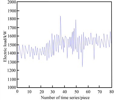
The historical load data collection results of the power system are shown in Fig. 3.

Fig. 2Weather data collection results

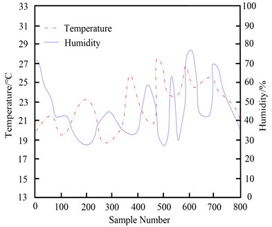
Fig. 3Historical load data

The proposed online sequential extreme learning support vector regression algorithm is applied to forecast power loads in the study area from July 1 to July 9, 2023, with the prediction results illustrated in Fig. 4.

Fig. 4 demonstrates that the proposed online sequential extreme learning support vector regression algorithm achieves short-term power load forecasts closely matching actual measurements. These results validate the method's ability to generate accurate predictions, establishing a reliable foundation for subsequent load interval estimation.

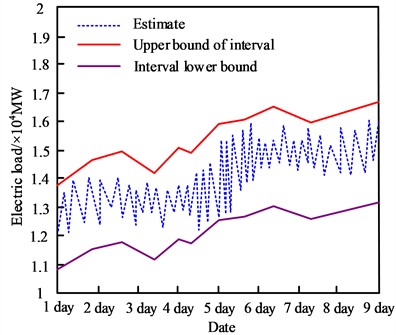
Based on the short-term power load forecasting results, power load interval estimation is conducted, and the estimation results are shown in Fig. 5.

Fig. 5 demonstrates that the proposed method, building upon short-term load forecasting results from the online sequential extreme learning support vector regression algorithm, effectively generates power load interval estimates. From an operational perspective, load interval estimation provides comprehensive information for power system dispatch. Operators can optimize generation scheduling and unit commitment based on interval boundaries, ensuring both grid stability and economic efficiency. For electricity market participants, accurate interval forecasting enables more informed trading strategies and reduced market exposure.

Fig. 4Short term power load forecasting results

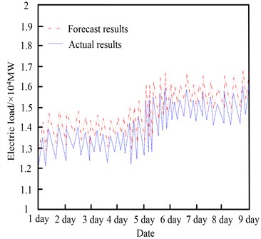
Fig. 5Estimation results of power load interval

To quantitatively analyze the contributions of the three core design components in the OS-ELM-SVR framework (dynamic features, SVR regressor, dynamic interval estimation), the following ablation variant models for controlled variable experiments are designed:

SF-SVR (Static Feature SVR): Removes dynamic features. Trains a static SVR model using original static features (time, temperature, etc.), which remains unchanged across the entire test set. This experiment evaluates the value of OS-ELM's dynamic feature generation.

OS-ELM (Linear): Removes the SVR regressor. Performs online prediction using standard OS-ELM (linear output layer) only. This experiment assesses the value of introducing a nonlinear SVR regressor.

OS-ELM-SVR (Static Interval): Remove dynamic interval estimation. Perform point predictions using the full OS-ELM-SVR model, but construct intervals using globally fixed error quantiles computed over the entire training set instead of dynamically updated distributions over time. This experiment evaluates the value of dynamically updating error distributions.

Proposed (Full Model): The complete model. This combines OS-ELM-SVR with the conditional compliance prediction (CP) framework.

Experimental results are shown in Table 2.

Table 2Performance comparison of ablation experiments (95 % confidence level)

Model Variants	RMSE (MW)	MAPE (%)	PICP (%)	PINAW (MW)
SF-SVR (Static Features)	278.4 ± 5.8	2.15 ± 0.07	94.0 ± 0.6	162.5 ± 4.0
OS-ELM (Linear Output)	268.2 ± 6.3	2.05 ± 0.08	92.8 ± 0.8	159.8 ± 4.5
OS-ELM-SVR (Static Intervals)	237.1 ± 3.6	1.81 ± 0.04	93.1 ± 0.7	156.3 ± 3.9
Proposed (Full Model)	236.7 ± 3.5	1.80 ± 0.04	94.5 ± 0.4	148.7 ± 3.5

As shown in Table 2, SF-SVR significantly underperforms the full model across all metrics, indicating that fixed features cannot adapt to the time-varying characteristics of load patterns. Dynamic feature updates are crucial for maintaining long-term prediction performance. OS-ELM (Linear) exhibits markedly higher point prediction errors, confirming the limitations of a single linear output layer in fitting complex nonlinear dynamics. Introducing kernel-based SVR significantly improves accuracy. OS-ELM-SVR (Static Interval) achieves point prediction accuracy comparable to the full model, but exhibits lower probability-of-interval coverage (PICP) and wider probability-of-interval width (PINAW). This indicates that using static historical error distributions fails to accurately reflect the evolving prediction uncertainty during online learning, resulting in intervals that are either under-covering or inefficient. Dynamic error distribution updates generate more precise and efficient prediction intervals.

In summary, ablation experiments quantitatively validate the effectiveness of each core design in this approach: dynamic feature updates ensure model adaptability, the SVR regressor enhances expressive power, and dynamic interval estimation optimizes uncertainty quantification quality. Their synergistic collaboration forms the foundation for the algorithm's superior performance in short-term electricity load point prediction and interval estimation tasks.

Two indicators are selected to evaluate the results of power load interval estimation: the coverage rate of the prediction interval and the width of the interval. Not only should the estimated interval have sufficient coverage, but it should also be as narrow as possible. The calculation formulas for each evaluation indicator are as follows:

(1) The calculation formula for the interval coverage rate $C P$ is as follows:

30

C P = \frac{M^{(1 - υ)}}{N} \times 100 %,

where, $N$ is the number of samples, and $M^{(1 - α)}$ is the number of actual values falling within the predicted confidence interval at the confidence level $1 - υ$ . $1 - υ$ is an important indicator for measuring interval prediction, statistically representing the proportion of actual values within the interval. The larger its value is, the higher the credibility.

(2) The calculation formula for the average width of the interval MWP is as follows:

31

M W P = \frac{1}{N} \sum_{i = 1}^{N} \frac{{\hat{L}}_{m a x} (x_{i}) - {\hat{L}}_{m i n} (x_{i})}{L_{a}},

where, $M W P$ is the interval average width at the confidence level $1 - υ$ ; ${\hat{L}}_{m a x} (x_{i})$ is the upper bound of the $i$ th predicted sample; ${\hat{L}}_{m i n} (x_{i})$ is the lower bound of the $i$ th predicted sample; $L_{a}$ is the actual value of the $i$ th sample. MWP is used to measure the ability of the interval to contain uncertain information, and a smaller value is better.

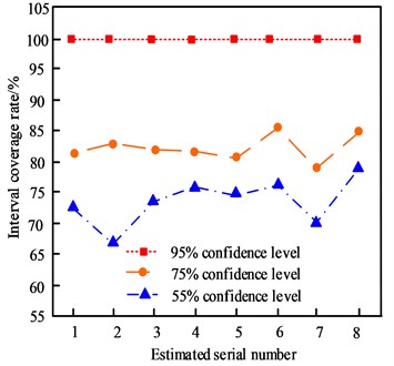
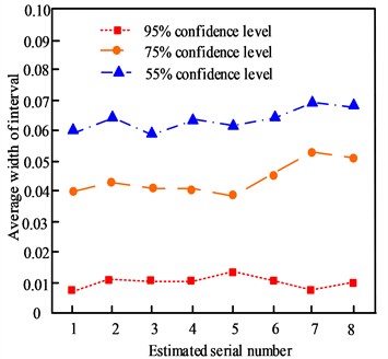
The statistics use the algorithm in this paper to estimate the interval coverage rate and average width of short-term power load, with the results shown in Fig. 6.

As shown in Fig. 6(a), the actual coverage rate corresponding to the 95 % confidence level is approximately [92-94] %, which, though slightly below the nominal confidence level, demonstrates good calibration properties. The coverage rates for the 75 % and 55 % confidence levels fluctuate around [70-80] % and [50-60] %, respectively. Fig. 6(b) shows that the average interval width increases with higher confidence levels, consistent with theoretical expectations - greater uncertainty requires wider intervals for adequate coverage. At the 95 % confidence level, the interval width remains within a reasonable range and does not approach zero. Combining Figs. 6(a) and (b) reveals that the proposed method achieves a good balance between coverage and interval width at the 95 % confidence level. It provides load fluctuation range information for system scheduling that is both highly reliable and not overly conservative. To further evaluate the calibration quality of the intervals, a probability integral transform (PIT) histogram is plotted. Fig. 6(c) shows that the PIT values exhibit a roughly uniform distribution, indicating that the empirical distribution of the prediction intervals aligns well with the distribution of actual loads. This confirms that the prediction intervals constructed based on the empirical distribution of dynamic errors possess good calibration characteristics, meaning their derived confidence levels largely match the empirical coverage probability without significant systematic bias toward being overly tight or overly loose.

Statistics are employed to estimate the short-term load intervals of this power system using the algorithm in this paper, the method from Reference [6] (Control Group 1), and the method from Reference [7] (Control Group 2). The voltage value changes in the power system are shown in Fig. 7.

Fig. 6Load interval estimation performance

a) Interval coverage rate

b) Average width of interval

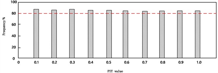
c) Histogram of probability integral transforms

Fig. 7Voltage variation in power system.

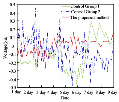
Analysis of Fig. 7 reveals that both the methods in Reference [6] and Reference [7] exhibit significantly larger voltage fluctuation ranges than the method proposed herein. During certain periods, fluctuations approach ±0.6 p.u. and ±0.8 p.u., respectively. Notably, the method in Reference [7] demonstrates the most severe voltage fluctuations, with maximum amplitude exceeding [specific value], accompanied by persistent undervoltage conditions. This indicates that their load forecasting intervals may suffer from coverage gaps or excessive conservatism during certain periods. Consequently, dispatch decisions fail to fully counteract voltage disturbances caused by load variations. The forecasting intervals thus inadequately capture the actual load fluctuation range, rendering the dispatch plan incapable of ensuring voltage quality. Under the algorithm applied in this paper, voltage fluctuations are strictly controlled within ±0.4 p.u., exhibiting the smoothest curve without significant voltage drops or out-of-limit events. This indicates that scheduling decisions based on the algorithm's precise load interval predictions help maintain system voltage stability and enhance operational quality. This is because the proposed method achieves both high coverage and narrow width in the prediction interval by leveraging the dynamic feature adaptability of OS-ELM and the strong nonlinear fitting capability of SVR. High coverage ensures the load fluctuation range perceived by the dispatch system sufficiently encompasses most practical scenarios, preventing insufficient reserve capacity due to “underreporting.” Narrow width enables more precise quantification of uncertainty, avoiding excessive allocation of costly regulation resources due to “overreporting.” This synergy allows dispatch commands to simultaneously ensure safety and pursue economy, ultimately manifesting as a stable voltage curve.

To comprehensively evaluate the performance of the proposed OS-ELM-SVR framework, we compare it against five categories of powerful and widely used benchmark models spanning statistical learning, machine learning, deep learning, and specialized interval forecasting methods:

Statistical models: SARIMA (Seasonally Autoregressive Integrated Moving Average), ETS (Exponential Smoothing Time Series).

Classic Machine Learning Models: LightGBM [citation], Standard Support Vector Regression (SVR), Gradient Boosting Quantile Regression (QB-GBM).

Online/Sequential Learning Models: Standard OS-ELM (linear output layer only), Online Kernel Learning (NORMA).

Deep Learning Methods: LSTM, Time Convolutional Network (TCN), Transformer.

Specialized interval prediction methods: Quantile Random Forest (QRF), LSTM with Conditional Probability Forecasting (LSTM+CP).

All models employ identical training, validation, and testing data splits, input features, and rolling prediction protocols. Point prediction and interval prediction performance are evaluated separately.

The point prediction performance comparison results for various methods are shown in Table 3.

Table 3Comparison of short-term electricity load point prediction performance among different models

Model category	Specific model	RMSE (MW)	MAPE (%)	Average single-step prediction time (ms)
Statistical models	SARIMA	312.5 ± 8.2	2.45 ± 0.10	1.2
Statistical models	ETS	298.7 ± 7.5	2.32 ± 0.08	0.8
Machine learning	LightGBM	241.3 ± 4.1	1.85 ± 0.05	0.5
Machine learning	Standard SVR	278.4 ± 5.8	2.15 ± 0.07	1.0
Online learning	Standard OS-ELM	268.2 ± 6.3	2.05 ± 0.08	0.3
Deep learning	LSTM	245.8 ± 12.5	1.88 ± 0.15	15.2
	TCN	243.1 ± 10.8	1.86 ± 0.12	8.7
	Transformer	240.5 ± 11.0	1.84 ± 0.11	22.5
Methodology	OS-ELM-SVR	236.7 ± 3.5	1.80 ± 0.04	1.8

As shown in Table 3, the proposed OS-ELM-SVR framework achieves the best performance in both RMSE and MAPE, with the smallest standard deviation, demonstrating excellent prediction accuracy and stability. Its accuracy surpasses all single models, including the expressive Transformer and the efficient LightGBM. Compared to standalone OS-ELM, the accuracy significantly improves when combined with SVR, validating the necessity of the nonlinear regression component. In computational efficiency, while our method is less efficient than OS-ELM and LightGBM, it is significantly faster than deep learning models, achieving a favorable balance between accuracy and efficiency.

The results of interval prediction performance comparison (95 % confidence level) are shown in Table 4.

Table 4Comparison of short-term electricity load interval prediction performance among different models (95 % confidence level)

Model	PICP (%)	PINAW (MW)	Interval Score (IS)
QB-GBM	94.8 ± 0.6	158.3 ± 4.2	142.1
Quantile Random Forest (QRF)	96.1 ± 0.5	172.5 ± 5.1	165.3
LSTM+CP	95.2 ± 0.3	155.0 ± 3.8	138.5
The Method in This Paper (OS-ELM-SVR-CP)	94.5 ± 0.4	148.7 ± 3.5	133.2

As shown in Table 4, to ensure fairness and theoretical robustness in interval prediction, this paper employs the Conditional Conformal Prediction (CP) framework to construct prediction intervals for all point prediction models (including the proposed method, LSTM, and LightGBM). Our method (OS-ELM-SVR-CP) achieves the narrowest mean interval width (PINAW) and the optimal interval synthesis score (IS) while reaching an approximate nominal coverage rate (~95 %), indicating that the generated prediction intervals are more precise and efficient. This advantage stems from OS-ELM-SVR's more precise point predictions, which reduce overall uncertainty and enable the CP framework to construct tighter reliable intervals.

4. Conclusions

This paper proposes a short-term power load interval estimation algorithm integrating Online Sequential Extreme Learning Machine (OS-ELM), Support Vector Regression (SVR), and dynamic error distribution. By synergizing OS-ELM's online feature evolution mechanism with SVR's robust nonlinear modeling capability, this framework effectively addresses dynamic adaptation and precise forecasting of load data streams while delivering reliable probabilistic interval outputs. Key contributions and conclusions are as follows:

1) A dynamically collaborative prediction architecture is proposed, demonstrating significantly superior performance compared to single models or static ensemble methods. Ablation experiments demonstrate that dynamic feature updates reduce RMSE from 278.4 MW to 237.1 MW; incorporating the SVR nonlinear regressor further lowers RMSE from 268.2 MW to 236.7 MW; while the dynamic interval estimation mechanism optimizes the average interval width from 156.3 MW to 148.7 MW while maintaining high coverage.

2) Demonstrated quantitative advantages in both point and interval forecasting. For point forecasting, our method achieved lower RMSE (236.7 MW) and MAPE (1.80 %) than all comparison models, with the smallest standard deviation, showcasing excellent accuracy and stability. For interval prediction, the method achieves 94.5 % coverage at the 95 % confidence level with the narrowest interval width (148.7 MW). Its Integrated Score (IS) of 133.2 outperforms specialized interval prediction methods such as quantile random forest, QB-GBM, and LSTM+CP.

3) Demonstrated clear engineering applicability and economic value. The algorithm's precise interval predictions provide comprehensive decision support for power system dispatch, aiding in more economical generation scheduling and reserve capacity allocation. Simulations show that applying this algorithm effectively suppresses system voltage fluctuations within ±0.4 p.u., significantly outperforming traditional prediction methods and reducing operational risks and costs. Additionally, the algorithm exhibits high computational efficiency, making it suitable for online deployment. It provides reliable technical support for real-time grid dispatch and market transactions under high renewable energy penetration.

Although the OS-ELM-SVR framework proposed in this study demonstrates excellent dynamic forecasting and interval estimation performance under high-volatility summer load scenarios, the work still has certain limitations. For instance, electricity loads exhibit significant long-term seasonal patterns (such as winter heating and spring/autumn transitions), and the current results have not undergone long-term stability testing across full annual cycles or seasonal transitions. Future research should conduct systematic validation using larger datasets encompassing multiple seasons and varying climatic years.

References

V. Veeramsetty, K. R. Reddy, M. Santhosh, A. Mohnot, and G. Singal, “Short-term electric power load forecasting using random forest and gated recurrent unit,” Electrical Engineering, Vol. 104, No. 1, pp. 307–329, Aug. 2021, https://doi.org/10.1007/s00202-021-01376-5

Publisher
A. Saeed, C. Li, Z. Gan, Y. Xie, and F. Liu, “A simple approach for short-term wind speed interval prediction based on independently recurrent neural networks and error probability distribution,” Energy, Vol. 238, No. Jan.1 Pt.C, p. 122012, Jan. 2022, https://doi.org/10.1016/j.energy.2021.122012

Publisher
M. Hanif, M. K. Shahzad, V. Mehmood, and I. Saleem, “Epfg: electricity price forecasting with enhanced gans neural network,” IETE Journal of Research, Vol. 69, No. 9, pp. 6473–6482, Sep. 2023, https://doi.org/10.1080/03772063.2021.2000510

Publisher
A. Rafati, M. Joorabian, E. Mashhour, and H. R. Shaker, “Machine learning-based very short-term load forecasting in microgrid environment: evaluating the impact of high penetration of PV systems,” Electrical Engineering, Vol. 104, No. 4, pp. 2667–2677, Feb. 2022, https://doi.org/10.1007/s00202-022-01509-4

Publisher
S. Özen, A. Yazıcı, and V. Atalay, “Hybrid deep learning models with data fusion approach for electricity load forecasting,” Expert Systems, Vol. 42, No. 2, pp. e13741.1–e13741.31, Sep. 2024, https://doi.org/10.1111/exsy.13741

Publisher
N. Bashiri Behmiri, C. Fezzi, and F. Ravazzolo, “Incorporating air temperature into mid-term electricity load forecasting models using time-series regressions and neural networks,” Energy, Vol. 278, No. Sep.1, p. 127831, Sep. 2023, https://doi.org/10.1016/j.energy.2023.127831

Publisher
M. R. N. Kalhori, I. T. Emami, F. Fallahi, and M. Tabarzadi, “A data-driven knowledge-based system with reasoning under uncertain evidence for regional long-term hourly load forecasting,” Applied Energy, Vol. 314, No. May 15, p. 118975, May 2022, https://doi.org/10.1016/j.apenergy.2022.118975

Publisher
M. Chauhan, S. Gupta, and M. Sandhu, “Short-term electric load forecasting using support vector machines,” ECS Transactions, Vol. 107, No. 1, pp. 9731–9737, Apr. 2022, https://doi.org/10.1149/10701.9731ecst

Publisher
F. Bayram, P. Aupke, B. S. Ahmed, A. Kassler, A. Theocharis, and J. Forsman, “DA-LSTM: a dynamic drift-adaptive learning framework for interval load forecasting with LSTM networks,” Engineering Applications of Artificial Intelligence, Vol. 123, No. Pt.C, p. 106480, Aug. 2023, https://doi.org/10.1016/j.engappai.2023.106480

Publisher
X. F. Xu, Y. Zhao, M. Gong, and Y. L. Chen, “Short-term power load forecasting based on dimensionality reduction and combined model,” (in Chinese), Computer Simulation, Vol. 39, No. 4, pp. 66–70, 2022, https://doi.org/10.3969/j.issn.1006-9348.2022.04.013

Publisher
M. Elkamel, A. Ahmadian, and Q. P. Zheng, “Impact of coronavirus disease 2019 on electricity demand and the unit commitment problem: a long-short-term memory-based machine learning approach,” Engineering Optimization, Vol. 54, No. 11, pp. 1835–1852, Nov. 2022, https://doi.org/10.1080/0305215x.2021.1961762

Publisher
S. S. Subbiah and J. Chinnappan, “Deep learning based short term load forecasting with hybrid feature selection,” Electric Power Systems Research, Vol. 210, No. Sep., p. 108065, Sep. 2022, https://doi.org/10.1016/j.epsr.2022.108065

Publisher
M. López, C. Sans, and S. Valero, “Automatic classification of special days for short-term load forecasting,” Electric Power Systems Research, Vol. 202, No. Jan., p. 107533, Jan. 2022, https://doi.org/10.1016/j.epsr.2021.107533

Publisher
A. O. Aseeri, “Effective rnn-based forecasting methodology design for improving short-term power load forecasts: application to large-scale power-grid time series,” Journal of Computational Science, Vol. 68, No. Apr., p. 101984, Apr. 2023, https://doi.org/10.1016/j.jocs.2023.101984

Publisher
G. Gürses-Tran, T. A. Körner, and A. Monti, “Introducing explainability in sequence-to-sequence learning for short-term load forecasting,” Electric Power Systems Research, Vol. 212, p. 108366, Nov. 2022, https://doi.org/10.1016/j.epsr.2022.108366

Publisher
R. Panigrahi, N. R. Patne, B. V. Surya Vardhan, and M. Khedkar, “Short-term load analysis and forecasting using stochastic approach considering pandemic effects,” Electrical Engineering, Vol. 106, No. 3, pp. 3097–3108, Dec. 2023, https://doi.org/10.1007/s00202-023-02135-4

Publisher
T. Ahmad and D. Zhang, “A data-driven deep sequence-to-sequence long-short memory method along with a gated recurrent neural network for wind power forecasting,” Energy, Vol. 239, p. 122109, Jan. 2022, https://doi.org/10.1016/j.energy.2021.122109

Publisher
R. Keshvari, M. Imani, and M. Parsa Moghaddam, “A clustering-based short-term load forecasting using independent component analysis and multi-scale decomposition transform,” The Journal of Supercomputing, Vol. 78, No. 6, pp. 7908–7935, Jan. 2022, https://doi.org/10.1007/s11227-021-04195-4

Publisher
L.-G. Maltais and L. Gosselin, “Forecasting of short-term lighting and plug load electricity consumption in single residential units: development and assessment of data-driven models for different horizons,” Applied Energy, Vol. 307, No. Feb.1, p. 118229, Feb. 2022, https://doi.org/10.1016/j.apenergy.2021.118229

Publisher
O. Trull, J. C. García-Díaz, and A. Peiró-Signes, “MSF, a forecasting library to predict short-term electricity demand based on multiple seasonal time series,” Journal of Computational Science, Vol. 78, No. Jun., p. 102280, Jun. 2024, https://doi.org/10.1016/j.jocs.2024.102280

Publisher

About this article

Received

September 5, 2025

Accepted

April 9, 2026

Published

September 27, 2026

DOI

https://doi.org/10.21595/jme.2026.25355

Keywords

online sequential learning

extreme learning machine

support vector regression

short-term load forecasting

interval estimation

dynamic characteristics

Acknowledgements

The authors have not disclosed any funding.

Data Availability

The datasets generated during and/or analyzed during the current study are available from the corresponding author on reasonable request.

Author Contributions

Yaxing Wei: writing-original draft preparation; Jiamao Han: writing-review and editing; Bin Zhao: formal analysis; Yujia Chen: investigation; Wei Ao: methodology; Mingzuo Ma: supervision; Lai Man: Conceptualization. All authors have read and agreed to the published version of the manuscript.

Conflict of interest

The authors declare that they have no conflict of interest.

This is an open access article distributed under the Creative Commons Attribution License (CC BY 4.0), which permits unrestricted use, distribution, and reproduction in any medium, provided the original work is properly cited.