A cross-domain fault diagnosis method for vehicle motors under variable operating conditions based on attention-guided graph convolutional networks

1. Introduction

Electric vehicles, as the core carriers of modern road transportation, play a vital role in national economic development, logistics systems, and low-carbon policies. With the continuous increase in vehicle ownership and mileage, higher demands are placed on driving safety, stability, and operational efficiency. As the core component of an electric vehicle’s powertrain, the health status of the motor directly determines driving safety, power output stability, and range capability. However, unlike controlled laboratory settings, in-vehicle motors are routinely exposed to sustained high-load operation, complex road-induced vibrations, and frequent start-stop transients, leading to strongly time-varying operating conditions and non-stationary, interference-prone monitoring signals. Under such variable operating conditions, the probability of failures occurring in internal components such as windings, bearings, and rotors significantly increases [1]. More importantly, these coupled variations in operating regimes and signal quality widen the practical gap for fault diagnosis: diagnostic models must remain accurate and reliable when conditions drift in real driving scenarios. Therefore, conducting precise fault diagnosis (FD) research on automotive motors under variable operating conditions is crucial for ensuring the safe and reliable operation of vehicles, preventing driving interruptions or even safety incidents caused by motor failures.

Data-driven intelligent methods have created new opportunities for FD, as they can automatically learn complex feature representations from large-scale data without relying on handcrafted feature design, thereby showing clear advantages in FD tasks [2-3]. For example, Zhang et al. [4] developed an integrated sparse supervision model based on sparse feature extraction, enabling efficient FD. Liu et al. [5] proposed a multi-domain CNN that achieves high-precision motor bearing diagnosis by jointly extracting one-dimensional and two-dimensional features. He et al. [6] constructed an FD approach for train traction motor bearings using multi-sensor data fusion, where deep and shallow features across different spatial dimensions are captured via a fused three-dimensional pixel matrix. Nevertheless, automotive motors typically operate under complex and highly variable conditions. The above methods often require time-consuming and labor-intensive data collection for each specific operating condition to train or calibrate models, which limits their practicality when operating conditions change frequently. Moreover, variations in operating regimes can induce pronounced, dynamic shifts in signal characteristics, making fault-related features harder to extract consistently and reliably. Consequently, FD models are confronted with stringent requirements in terms of generalization and adaptability under changing conditions.

Cross-domain diagnostics have become a current research hotspot due to their ability to infer and reflect the characteristic manifestations of identical faults under other operating conditions by leveraging common fault features extracted from partial operating condition data. For example, Kim et al. [7] proposed a preprocessing method for stator current operational compensation. By resampling and recalibration, each learning sample was made to contain the same electrical angle period, and amplitude differences were equalized. This significantly mitigated distribution drift caused by operating condition variations such as speed and torque, thereby improving the robustness and accuracy of PMSM FD under multiple operating conditions. Li et al. [8] proposed a knowledge mapping-based adversarial domain adaptation method. Within an adversarial learning framework, it combines discriminative feature distance metrics with auxiliary classifiers. By utilizing a knowledge mapping module to extract domain-invariant features, the approach significantly reduces the distributional differences between the source and target domains under varying operating conditions. Zhu et al. [9] proposed a FD method for variable operating conditions. It first converts vibration signals into vibration images to fully characterize time-frequency and texture information, then constructs a domain-adaptive network to perform alignment at both global and subdomain levels. This approach achieves high-accuracy, strong-generalization intelligent diagnostic performance across multiple operating conditions. However, during vehicle operation, the motor faces multi-source coupled excitation, causing the acquired signals to suffer from noise interference. The aforementioned methods struggle to effectively address diagnostic tasks under varying noise conditions. Furthermore, the accurate extraction of cross-domain features remains a significant challenge. Conventional FE methods struggle to adapt effectively to the dynamic operating conditions encountered during vehicle operation, resulting in low diagnostic accuracy.

CNNs have found extensive application in the field of FD due to their exceptional FE capabilities. Through the synergistic interaction of convolutional and pooling layers, CNNs can extract local features from fault data and progressively construct higher-level feature representations [10-12]. However, although CNNs are able to progressively build more global representations by stacking multiple convolutional layers, their feature extraction is still largely achieved by aggregating local receptive-field patterns. As a result, it can be difficult for CNN-based models to explicitly capture long-range dependencies and complex correlations embedded in the global information. In contrast, graph convolutional networks can naturally represent the underlying structure of samples as association graphs, where nodes and edges encode entities and their interactions. This graph-based formulation enables the model to directly model intricate relationships among sample data, and to more thoroughly explore the spatial dependencies and temporal dynamics within the data, leading to richer and more informative representations for downstream analysis. Therefore, GCNs can compensate for the shortcomings of CNNs and significantly enhance fault classification capabilities [13]. The core idea of GCNs is to update node feature representations by aggregating information from nodes and their neighbors, thereby capturing both global and local information within the graph structure to achieve outstanding performance [14-15]. In recent years, researchers have begun applying GCNs to the field of FD, achieving significant progress. Li et al. [16] proposed a multi-receptive field GCN that aggregates information from different neighborhoods using multi-receptive field graph convolutional layers. This approach achieved high-accuracy FD across multiple complex mechanical fault datasets and demonstrated excellent robustness under conditions of extreme sample imbalance. Cao et al. [17] introduced a novel pulse graph attention network for intelligent FD of planetary gearboxes, enabling simultaneous extraction of spatio-temporal features from gearbox signals. Yu et al. [18] proposed a two-stage importance-aware subgraph CNN based on multi-source sensors, enhancing the fault recognition performance of intelligent neural networks under variable conditions and limited data. Ma et al. [19] introduced a self-attention GCN employing fast local spectral filters based on Legendre polynomials and self-attention graph pooling methods, significantly improving model stability and computational efficiency. Han et al. [14] proposed a complex industrial process FD method based on multi-relational fusion GCN and multi-scale residual networks, effectively handling multi-scale temporal correlation features and comprehensively representing complex relationships among sensors. Evidently, graph neural networks hold immense promise for fault diagnosis in complex systems. By explicitly modeling the structured relationships among multiple sensing channels and components, they can more comprehensively uncover latent fault characteristics both across signals and within individual signals. This capability enables the construction of more accurate, discriminative, and interpretable feature representations, thereby providing a solid foundation for reliable and precise subsequent diagnostic decision-making.

Although the existing data-driven and cross-domain fault diagnosis methods have achieved satisfactory results, they still face several significant challenges in real automotive motor diagnosis, including insufficient adaptability to rapidly changing operating conditions, limited robustness under noise interference, and insufficient ability to extract global structural features from complex monitoring signals. These limitations hinder reliable fault diagnosis in actual driving scenarios. To address these issues, this study explores cross-domain fault diagnosis of automotive motors under changing operating conditions and proposes an attention-guided graph convolutional network (AGGCN) to achieve more robust feature representation and more accurate fault classification. The main contributions of this study are summarized as follows:

(1) A method combining time-frequency domain feature fusion with wavelet kernel convolution is proposed to achieve deep extraction of signal features in noisy environments.

(2) To address the challenge of FE in cross-domain diagnostics under variable OC, a fusion approach is proposed. It integrates a graph generation structure based on attention mechanisms, autoregressive moving average filter graph convolutions, and a multi-order GCN based on Chebyshev polynomials. This enhances FE capabilities and effectively captures multi-scale information.

(3) Integrating the aforementioned approaches forms a graph convolutional-based cross-domain FD method, whose reliability is validated using the GXU motor fault dataset.

2. Background information

2.1. ARMA graph convolution

Auto-regressive moving average (ARMA) graph convolution [20] is implemented based on auto-regressive moving average filters. Compared to polynomial graph convolutions, such as Chebyshev graph convolutions, ARMA graph convolutions offer more flexible frequency responses, capture better graph-global structures with fewer parameters, and exhibit superior noise resistance against noise in graph signals. The operation of ARMA filters is illustrated as follows:

Its frequency response formula is:

1

$h_{ARM{A}_K}\left(\lambda \right)=\frac{{\sum }_{k=0}^{K-1}{p}_k{\lambda }^k\hspace{0.33em}}{1+{\sum }_{k=1}^K{q}_k{\lambda }^k\hspace{0.33em}},$

where, $K$ denotes the order of the filter, $\lambda$ represents the eigenvalues of the Laplace matrix, $p_k$ and $q_k$ are the filter coefficients that are automatically updated through training, and $I$ is the identity matrix used to preserve the dimensions and structure of the matrix.

In the node space, the filtering relationship of the ARMA filter is:

2

$\bar{X}={\left(I+\sum _{k=1}^K{q}_k{L}^k\right)}^{-1}\left({\sum }_{k=0}^{K-1}{p}_k{L}^k\right)X,$

where, $L$ is the symmetric normalized Laplacian matrix (LM) of the graph, $X$ is the graph signal, and $\stackrel{-}{X}$ is the filtered graph signal.

ARMA filters are implemented through recursive approximation. For a first-order ARMA filter, the recursive update formula is:

3

${\bar{X}}^{(t+1)}=aM{\bar{X}}^{\left(t\right)}+bX,$

4

$M=\frac{1}{2}\left({\lambda }_{max}-{\lambda }_{min}\right)I-L,$

where, ${\lambda }_{max}$ and ${\lambda }_{min}$ represent the maximum and minimum eigenvalues of the Laplace matrix, $a$ and $b$ denote learnable parameters, and $t$ indicates the number of recursive iterations.

Then, based on the convergence of Eqs. (4-6), the frequency response of a first-order ARMA filter can be defined as:

5

$\bar{X}=\underset{t\to \infty }{\mathrm{l}\mathrm{i}\mathrm{m}}\left[(aM{)}^t{X}^{\left(0\right)}+b{\sum }_{i=0}^t(aM{)}^{i}X\right].$

Among them, the eigenvectors of $M$ and Lare identical, but their eigenvalues differ. If ${\mu }_m$ is an eigenvalue of $M$ and ${\mu }_l$ is an eigenvalue of $L$, then the relationship is as follows:

6

${\mu }_m=\frac{1}{2}\left({\lambda }_{max}-{\lambda }_{min}\right)-{\mu }_l.$

Let ${\mu }_m\in [-\mathrm{1,1}]$, when $\left|a\right|<1$, the first term is:

7

$\underset{t\to \infty }{\mathrm{l}\mathrm{i}\mathrm{m}}(aM{)}^t=0.$

The second item is expressed as:

8

$\underset{t\to \infty }{\mathrm{l}\mathrm{i}\mathrm{m}}\left(b{\sum }_{i=0}^t(aM{)}^{i}X\right)=b(I-aM{)}^{-1}.$

Therefore, the frequency response of a first-order ARMA filter is:

9

$h_{ARM{A}_1}\left({\mu }_m\right)=\frac{b}{1-a{\mu }_m}.$

By summing K first-order ARMA filters, the analytical form of the ARMAK filter can be recovered. The filtering operation is:

10

$\bar{X}\hspace{0.33em}=\hspace{0.33em}{\sum }_{k=1}^K{\sum }_{m=1}^M\frac{b_k}{1-a_k{\mu }_m}{u}_m{u_m}^{T}X\hspace{0.33em},$

11

$h_{ARM{A}_k}\left({\mu }_m\right)={\sum }_{k=1}^K\frac{b_k}{1-a_k{\mu }_m},$

where, $u_m$ denotes the $m$th eigenvector of the graph’s LM $L$.

By setting coefficient $a_k$ to zero, the ARMA filter is converted into a polynomial filter.

Furthermore, by the recursive formula, the ARMA graph convolution is defined as:

12

$X^{(t+1)}=\sigma \left(L^{\text{'}}{X}^{\left(t\right)}W+XV\right),$

where, $\sigma$ is the activation function, $X$ is the initial node feature, $X$ and $V$ are trainable parameters, and $L^{\text{'}}$ is the modified LM, which is appropriately simplified by setting ${\lambda }_{min}=0$ and ${\lambda }_{max}=2$.

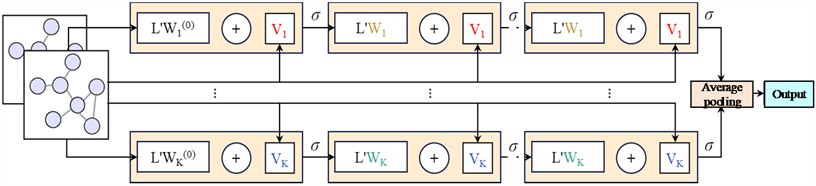
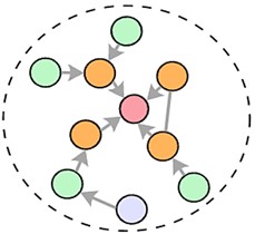
The ARMA graph convolutional architecture is shown in Fig. 1, where identical colors indicate weight sharing.

Fig. 1Workflow diagram of the ARMA graph convolution architecture

2.2. Chebyshev graph convolutions

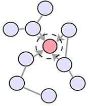
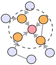
This model employs Chebyshev graph convolutions of varying orders [16] to capture multi-scale features within the graph. The feature update process for multi-order Chebyshev graph convolutional nodes is illustrated in Fig. 2. The parameter $K$ specifies the degree of the Chebyshev polynomial used in the convolution process. When $K=1$, the convolution kernel primarily focuses on a node’s first-order neighbors. When $K=$2, the kernel considers both first- and second-order neighbors, and so on.

Chebyshev graph convolutions approximate spectral graph convolutions using Chebyshev polynomials. The principle is illustrated by Eqs. (13-15).

Graph convolution is based on the eigenvalue decomposition of the graph LM $L$. The definition of the LM $L$ is shown in Section 2.2.1. Graph convolution is expressed as:

13

$X^{\text{'}}=U{g}_{\theta }\left(\mathrm{\Lambda }\right)U^{T}X,$

where, $U$ is the matrix of eigenvectors of $L$, $\mathrm{\Lambda }$ is the matrix of eigenvalues, $g_{\theta }$ is the filter of the graph network, which is a function of the eigenvalues $\mathrm{\Lambda }$ of $L$ with respect to the parameter $\theta$, and $\theta$ is the vector of Fourier coefficients.

To improve computational efficiency, Chebyshev polynomial $T_k\left(x\right)$ is used to approximate $g_{\theta }$:

14

$g_{\theta }\left(\mathrm{\Lambda }\right)\approx {\sum }_{k=0}^{K-1}{\theta }_k{T}_k\left(\mathrm{\Lambda }\right),$

where, $K$ denotes the degree of the Chebyshev polynomial, and ${\theta }_k$ represents the learnable parameter.

The output of a Chebyshev GCN can be expressed as:

15

$X^{\text{'}}={\sum }_{k=0}^{K-1}{\theta }_k{T}_k\left(L\right)X.$

Fig. 2The convolution principle of Chebyshev polynomials of different orders

a)$K=1$

b)$K=2$

c)$K=3$

3. Methodology

3.2. Graph convolution neural network

This section proposes an attention-based graph generation method-the attention-mechanism graph generation layer (AGGL)-which enhances the modeling capability of graph neural networks for complex data relationships by dynamically constructing graph structures. AGGL incorporates the squeeze-and-excitation (SE) attention mechanism [21]. By learning importance weights across feature channels, the SE attention mechanism recalibrates features and calculates attention scores between nodes based on these calibrated features. Simultaneously, the introduction of self-loops and threshold control further enhances the robustness and flexibility of the graph structure. Subsequently, the features of each signal sample are treated as graph nodes, and attention scores and weights are dynamically computed based on feature relationships between nodes to generate the graph structure. Fig. 3 shows its specific structure.

Fig. 3Attention-based graph generation architecture

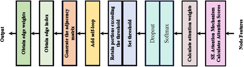
The SE attention mechanism first performs a Squeeze operation on the input features, compressing the channel dimension through global average pooling to extract global information. It then executes an Excitation operation, utilizing two fully connected (FC) layers and two nonlinear activation functions (ReLU and Sigmoid) to learn the importance weights for each channel, generating a weight vector. Finally, the learned weights are element-wise multiplied with the original features, amplifying important features while suppressing unimportant ones, yielding calibrated features.

The graph generation process based on the attention mechanism is as follows:

Attention scores are computed directly by the SE attention mechanism layer, where attention weights reflect the relationships between nodes. A random dropout layer reduces complex mutual adaptation among neurons, preventing overfitting:

16

$a=SEAttentio{n}_{ratio=16}\left(X\right),$

17

$A=Dropout\left(\mathrm{S}\mathrm{o}\mathrm{f}\mathrm{t}\mathrm{m}\mathrm{a}\mathrm{x}\left(a{a}^T\right)\right),$

Among these, $a$ is the attention score matrix, $a^T$ is its transpose matrix, $A$ represents the attention weights between nodes, and $SEAttention(\cdot )$ denotes the SE attention mechanism layer.

To reduce computational load while preserving critical information, an intensity threshold was set for sparsification. Self-loops were added to enhance nodes’ self-feature representations, thereby generating an adjacency matrix containing global information:

18

$\tilde{A}=\mathrm{t}\mathrm{h}\mathrm{r}\mathrm{e}\mathrm{s}\mathrm{h}\mathrm{o}\mathrm{l}\mathrm{d}\left(A\right)+I.$

Among these, $\tilde{A}$ represents the adjacency matrix considering self-loops, $\mathrm{t}\mathrm{h}\mathrm{r}\mathrm{e}\mathrm{s}\mathrm{h}\mathrm{o}\mathrm{l}\mathrm{d}(\cdot )$ denotes the threshold operation, in order to reduce the computational load while retaining the key structural information, a threshold operation will be performed on the adjacency matrix to achieve sparsification. The range of this value is usually 0.6-0.8. Following the values used in previous studies, in this research, the threshold has been empirically set to 0.7 [22, 23], and $I$ is the identity matrix containing the node's intrinsic features.

Finally, the edge weights and indices are extracted for subsequent operations. An ARMA layer is constructed based on ARMA filters to capture multi-scale features of nodes in the graph. This ARMA layer consists of two parallel branches, each containing three layers of ARMA filters (iterated three times), progressively extracting deeper-level features. Each branch learns two distinct filter responses, thereby capturing two sets of features at different scales. Subsequently, a residual connection sums the original features with the extracted features, enabling the model to converge more rapidly to a higher level of accuracy.

The Chebyshev graph convolutional layer is configured with $K$ set to 1, 2, and 3 to capture features at different scales [24, 25]. The detailed process of the complete multi-scale fusion graph convolutional layer is shown in Eqs. (19-25):

19

$edg{e}_{weight},edg{e}_{index}=AGGL\left(X\right),$

20

$X_{ARMA}=ARMACon{v}_{\left(K=2,T=3\right)}\left(X,edg{e}_{index},edg{e}_{weight}\right),$

21

$X^{\text{'}}=BatchNor{m}_1\left(X_{ARMA}\right),$

22

$\left\{\begin{array}{c}{X}_1=ChebCon{v}_{\left(K=1\right)}\left(X^{\text{'}}\right),\\ X_2=ChebCon{v}_{\left(K=2\right)}\left(X^{\text{'}}\right),\\ X_3=ChebCon{v}_{\left(K=3\right)}\left(X^{\text{'}}\right),\end{array}\right.$

23

$X_{Cheb}=Concat\left(X_1,X_2,X_3\right),$

24

$X^{\text{'}\text{'}}=BatchNorm2\left(X_{Cheb}\right),$

25

$X_{Output}=Dropout\left(ReLU\left(Linear\left(X^{\text{'}\text{'}}\right)\right)\right).$

Among these, $X$ represents the input sample signal, $X_{Output}$ indicates the features processed through the multiscale fusion graph convolution layer, while $edg{e}_{index}$ and $edg{e}_{weight}$ correspond to the edge connectivity information and weights of the adjacency graph obtained after passing through the graph generation layer AGGL.

Using cross-entropy loss to feed back classification loss, the classification loss function is expressed as follows:

26

$Los{s^C}_{total}=-\frac{1}{N_{total}}{\sum }_{i=1}^{N_{total}}\left({\sum }_{j=1}^N\{y_i=j\}\log \left(D_c\left(F\left(X_i\right)\right)\right)\right),$

where, $N_{total}$ represents the total sample size, $X_i$ denotes the input of the $i$th sample in category $j$, $F(\cdot )$ is the feature extractor, and $D_c(\cdot )$ is the classifier composed of a FC layer and a Softmax layer.$\{y_i=j\}$ indicates that if sample $i$ is estimated as belonging to class $j$, then $\{y_i=j\}=1$; otherwise, $X$ is 0.

Use adversarial networks to construct the loss function [26]. By minimizing the distributional difference between the source and target domains, the feature extractor generates domain-invariant features. Specifically, adversarial training is applied to the domain discriminator to distinguish whether data originates from the source or target domain. A binary cross-entropy loss function is then used to compute and minimize the discrepancy against the true labels. Finally, gradient reversal ensures the feature extractor and domain discriminator compete against each other, compelling the FE to generate features common to both domains.

The adversarial loss function is expressed as follows:

27

$Los{s^G}_{total}=-\frac{1}{N_{total}}{\sum }_{i=1}^{N_{total}}\left[\right(y_s\log (D_G\left(F_{si}\right))+((1-y_t)\log (D_G\left(F_{tj}\right)\left)\right],$

where, $N_{total}$ represents the total number of samples. $F_{si}$ and $F_{tj}$ denote the feature values extracted from samples in the source domain and target domain, respectively. $D_G(\cdot )$ is the domain discriminator. $y_s$ and $y_t$ indicate whether a sample is correctly predicted as belonging to the source domain or target domain; if so, they are 0, otherwise 1.

The total loss function is:

28

$Loss=Los{s^C}_{total}+Los{s^G}_{total}.$

3.3. FD process

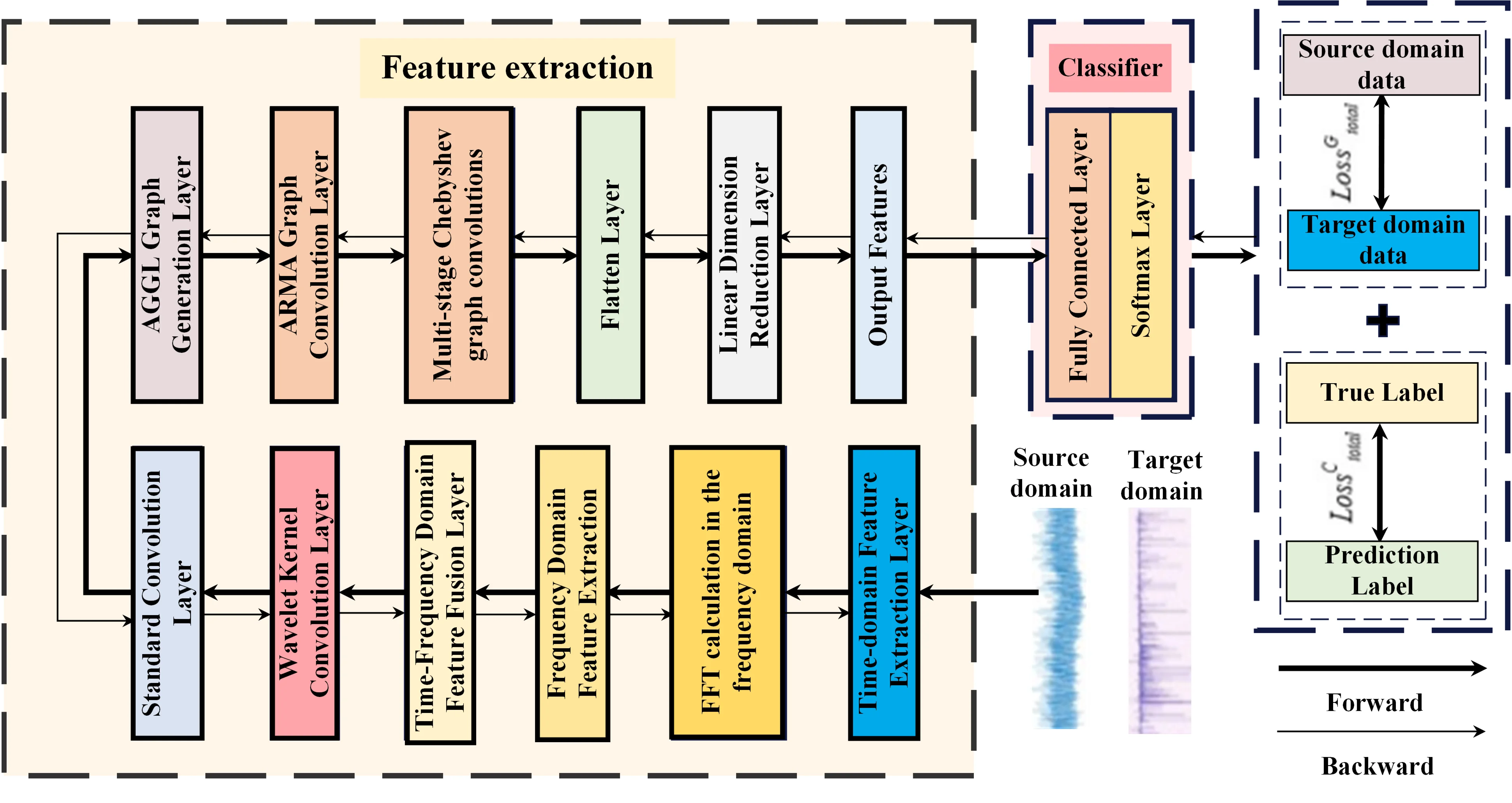
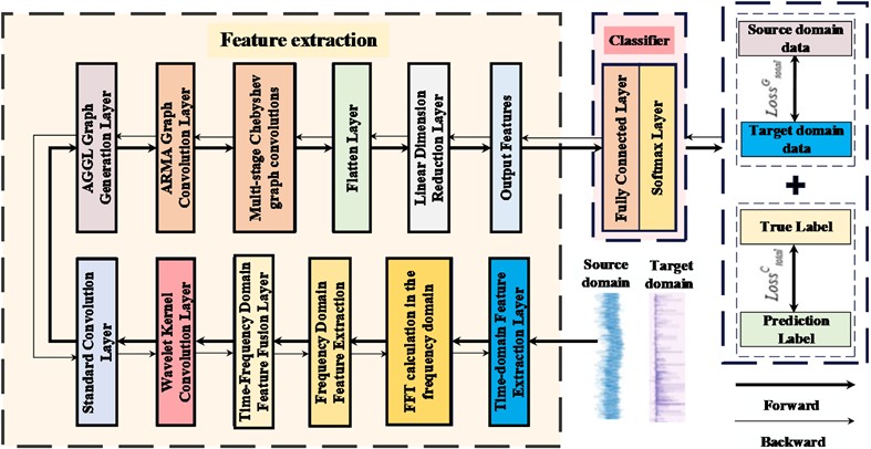
As shown in Fig. 4, this model first performs time-domain FE on the input signal, then converts the time-domain signal to the frequency domain through the FFT for FE, and then integrates it with the time-domain features. Subsequently, it undergoes deep FE using the wavelet kernel convolution layer and the ordinary convolution layer. Then, it passes through the input graph generation layer, the ARMA graph convolution layer, and the multi-order Chebyshev graph convolution layer to achieve further FE. Finally, it enters the subsequent classifier after passing through the flattening layer and the dimensionality reduction layer.

The signals collected by the sensors are labeled and randomly shuffled. The resulting samples are divided into training, validation, and test sets according to specific proportions. The AGGCN model parameters are trained and optimized using the training and validation samples. Finally, the trained model is employed as a pattern recognition algorithm for motor FD, with its overall diagnostic performance validated and analyzed through the test set.

Fig. 4The schematic diagram of the AGGCN fault diagnosis process proposed in this article

4. Experiments and results analysis

Because it is difficult for the motor to operate with faults for a long time in the vehicle, it makes it difficult to obtain real data. Therefore, this paper uses the data set collected from the experimental test bench to verify and compare the proposed finite element method based on graph convolution. This dataset originates from a motor fault simulation test bench manufactured by Guangxi university, designed for collecting simulated data on various motor faults. It is named the GXU Motor Fault Dataset. All experiments in this section and subsequent sections are implemented using the PyTorch framework and PyCharm software. The primary configuration of the experimental computer includes a GeForce RTX 3090 Ti graphics card with 24GB of VRAM and the Ubuntu 20.04 operating system.

4.1. Case study 1

4.1.1. Signal acquisition

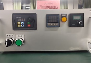
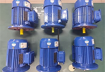
The GXU motor fault data acquisition device is shown in Fig. 5. This device comprises an GXU-F0.7 dynamometer, a hysteresis brake, and a fault motor. The hysteresis brake operates based on the principle of magnetic hysteresis, generating specific torque by adjusting the input excitation current. The motor fault types encompass the following seven categories: - Built-in bearing fault (outer ring raceway defect: width 0.5 mm × depth 0.3 mm) - Built-in imbalance fault - Built-in warping fault - Built-in static eccentricity fault - Built-in dynamic eccentricity fault - Built-in rotor bar breakage fault - Built-in bearing fault (rolling element defect: width 0.5 mm × depth 0.3 mm) The different motor fault types used in this experiment and their corresponding labels are shown in Table 1.

Fig. 5GXU motor multi-type fault data acquisition experimental platform. Photo by Zhenzhen Jin, Transportation Equipment Laboratory of the Mechanical Engineering College of Guangxi University, March 1st, 2025

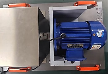
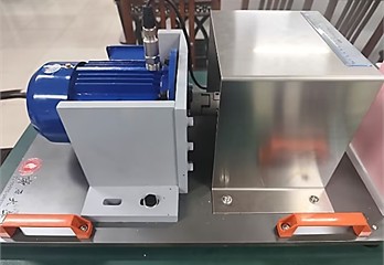
In this study, the operating conditions were varied by applying different load torque levels at a constant rotational speed. Therefore, this experiment mainly evaluated the cross-domain diagnostic performance of the proposed method under load variation conditions. Based on the torque corresponding to 0 %, 10 %, and 20 % of the rated excitation current (500 mA) at a rotational speed of 20 Hz, these conditions are defined as OC1, OC2, and OC3, respectively. The specific settings for different cross-domain diagnostic tasks are shown in Table 2. This model employs an end-to-end approach, directly feeding signal data from the dataset into the network for FE and classification. The signal data consists of one minute of sampled data after the motor stabilizes, with a sampling frequency of 20 kHz and a sample length truncated to 3072. After sliding window extraction, each fault type yields 325 samples. A total of seven faults were tested, resulting in 2275 samples per task. In the source domain data, 80 % is allocated for training and 20 % for validation. In the target domain data, 20 % is reserved for testing.

Table 1Seven types of motor failures and their corresponding labels

Label	Fault type	Fault explanation
0	Fault of the outer ring raceway	Damage has occurred to the raceway of the outer ring inside the bearing
1	Unbalanced fault	Uneven rotor mass distribution
2	Warpage fault	The rotor or shaft has become bent or deformed
3	Static eccentricity fault	The center of mass of the rotor is not on the axis of rotation
4	Eccentricity fault	The center of mass of the rotor shifts during rotation
5	Rotor bar breakage failure	A metal strip inside the rotor has fractured, resulting in uneven mass distribution
6	Bearing rolling element fault	The rolling elements inside the bearing have been damaged

Table 2Cross-domain diagnostic task

Task number	Source domain	Target domain
1	OC1	OC2
2	OC1	OC3
3	OC2	OC1
4	OC2	OC3
5	OC3	OC1
6	OC3	OC2

4.1.2. Cross-domain FD performance comparison analysis

To comprehensively evaluate the performance of the AGGCN model proposed in this chapter, five reference models were selected for comparison: Deep adversarial network for domain adaptation via backpropagation (DANN) [27]; Correlation-based alignment network for deep domain adaptation (CORAL) [28], Graph isomorphism network (GIN) [29], Domain-adversarial GCN under variable conditions (DAGCN) [30], Batch spectral penalty network for adversarial domain adaptation (BSP) [31]. AGGCN hyperparameters were set as follows: batch size 64, learning rate 0.001, training for 200 epochs, with gradient decay to 0.00001 starting from epoch 150. Hyperparameters for other models followed their original papers. Each method underwent five independent runs across all tasks to eliminate random variations and ensure result accuracy and reliability.

Table 3Comparison table of model FD accuracy under different operating conditions

Model Task	AGGCN	DANN	CORAL	GIN	DAGCN	BSP
1	96.39 %	94.20 %	83.84 %	86.84 %	62.72 %	51.56 %
2	93.71 %	90.48 %	77.53 %	70.03 %	64.91 %	53.75 %
3	98.25 %	94.05 %	80.21 %	91.08 %	61.11 %	65.50 %
4	93.12 %	89.73 %	90.03 %	75.73 %	69.01 %	64.06 %
5	97.22 %	90.48 %	78.72 %	81.55 %	54.66 %	29.38 %
6	96.49 %	92.26 %	91.82 %	78.95 %	58.77 %	27.81 %
Mean	95.86 %	91.87 %	83.69 %	80.70 %	61.86 %	48.68 %

As reported in Table 3, the proposed AGGCN achieves the best FD performance across all six cross-condition tasks, yielding a mean accuracy of 95.86 %. This result consistently surpasses the competing domain adaptation and graph-based baselines, including DANN (91.87 %), CORAL (83.69 %), GIN (80.70 %), DAGCN (61.86 %), and BSP (48.68 %), corresponding to improvements of 3.99, 12.17, 15.16, 34.00, and 47.18 percentage points, respectively. Notably, AGGCN maintains a high and stable accuracy range (93.12 %-98.25 %) under different transfer settings, indicating strong robustness to operating-condition variations. The comparative advantage suggests that merely aligning global feature distributions (e.g., DANN/CORAL) or relying on less adaptive relational modeling (e.g., GIN/DAGCN/BSP) may be insufficient when signal characteristics shift with speed/load changes. From a practical perspective, such consistent cross-condition performance implies that AGGCN can reduce the dependence on collecting and labeling large amounts of data for every single operating condition, thereby improving the feasibility of deploying FD models for automotive motors in real driving scenarios where operating regimes change frequently.

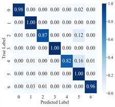
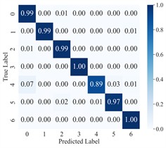
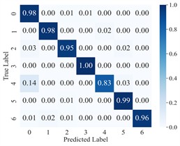
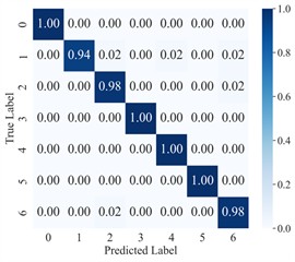
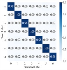
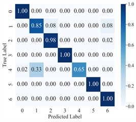
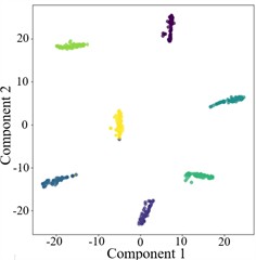
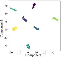
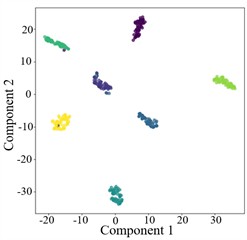
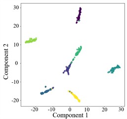
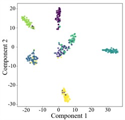
To more clearly demonstrate the model’s classification performance across different fault categories and to verify the effectiveness of feature extraction (FE), the diagnostic results of AGGCN are illustrated using a confusion matrix (Fig. 6) and t-SNE visualization (Fig. 7). As shown in these figures, Task 2 and Task 4 exhibit comparatively lower classification accuracy when operating conditions 1 and 2 are used for training and condition 3 is used for testing, whereas Task 5 and Task 6 achieve higher accuracy after swapping the training and testing sets. This performance asymmetry suggests that the discriminative characteristics among fault classes are less salient under lower-load regimes than under higher-load regimes. From a representation-learning perspective, lower loads typically lead to weaker fault excitations and reduced energy in fault-related components, which may compress inter-class feature distances and increase feature overlap, thereby making the decision boundaries less separable. In contrast, higher loads tend to intensify fault-induced responses and amplify subtle fault signatures, enabling the model to extract more distinctive and stable features and thus improving cross-condition generalization.

Fig. 6Confusion matrix of AGGCN under different task conditions

a) Task 1

b) Task 2

c) Task 3

d) Task 4

e) Task 5

f) Task 6

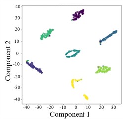
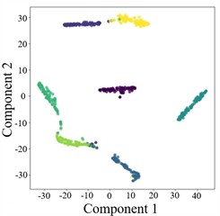
Moreover, the visualization results indicate that, regardless of the task setting, fault 3 consistently achieves 100 % classification accuracy, implying that its intrinsic signature is highly distinctive and forms a well-separated cluster in the learned feature space. By comparison, fault 4 presents a lower classification accuracy, which likely reflects a higher degree of similarity with other fault types and stronger susceptibility to operating-condition shifts and noise interference, causing partial cluster mixing in the embedding space and leading to misclassifications. This observation further highlights the importance of capturing fine-grained relational patterns and condition-invariant characteristics for confusing fault pairs, and it motivates deeper analysis of the extracted features (e.g., inter-class separability, intra-class compactness, and boundary samples). Overall, across a range of variable operating conditions, the proposed model maintains robust predictive performance and exhibits strong practical potential for real-world deployment.

Fig. 7T-SNE plots of AGGCN under different operating conditions and tasks

a) Task 1

b) Task 2

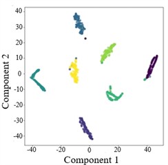
c) Task 3

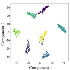
d) Task 4

e) Task 5

f) Task 6

4.1.3. Comparative analysis of cross-domain FD performance under noise conditions

The fault samples used in this experiment inherently contain a significant amount of noise. To fully extract shared features among samples within the same fault category, the experiments were conducted using operating conditions 1 and 2 as the training set and operating condition 3 as the test set. All other settings remained consistent with Section 4.1.2.

The signal-to-noise ratio is a metric that measures the ratio of the power of the useful signal to the power of the noise in a signal, typically expressed in decibels (dB). A higher signal-to-noise ratio indicates better signal quality relative to noise, meaning the signal is clearer. The formula for calculating the signal-to-noise ratio is shown in Eq. (29):

29

$SN{R}_{\left(dB\right)}=10\mathrm{l}\mathrm{o}{\mathrm{g}}_{10}\left(\frac{P_{signal}}{P_{noise}}\right).$

In the comparative analysis, the proposed AGGCN model employs a batch size of 64 and a learning rate of 0.001, with gradient decay to 0.00001 starting from the 150th epoch. Other models are configured according to the hyperparameters specified in the original paper. The training cycle spans 200 epochs. Each method underwent five tests across all tasks to mitigate random factors and ensure the accuracy and reliability of the results.

Table 4 further evaluates model robustness under increasingly severe noise. AGGCN exhibits strong noise tolerance, achieving 93.06 % at 0 dB and retaining 73.25 % even at –3 dB, whereas DANN and CORAL degrade dramatically (around 25 %-30 % under noisy settings), indicating that their distribution-alignment mechanisms are highly sensitive to heavy noise contamination. Compared with the graph baseline GIN, which remains relatively robust (87.57 % at 0 dB and 68.73% at −3 dB), AGGCN still provides a consistent margin, especially at low SNR (e.g., 73.25 % vs. 68.73 % at −3 dB). DAGCN shows moderate robustness but drops substantially as noise increases (59.80 %-39.62 %). These comparative results suggest that AGGCN is better at preserving discriminative fault information under noise interference, which is critical for in-vehicle environments where measurements are often affected by road excitation, electromagnetic interference, and sensor installation constraints. Practically, this robustness reduces the reliance on aggressive denoising or strict data-collection conditions, although the performance decline at extremely low SNR also indicates that improving sensor placement, sampling strategy, and lightweight preprocessing can further enhance real-world reliability.

Table 4Comparison table of FD accuracy rates in different noise environments

Model noise	AGGCN	DANN	CORAL	GIN	DAGCN
Noiseless	96.39 %	94.20 %	83.84 %	86.84 %	62.72 %
0 dB	93.06 %	29.84 %	27.50 %	87.57 %	59.80 %
–1 dB	87.03 %	29.53 %	27.66 %	86.70 %	50.88 %
–2 dB	83.04 %	28.44 %	26.25 %	79.50 %	47.37 %
–3 dB	73.25 %	27.97 %	25.47 %	68.73 %	39.62 %

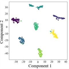
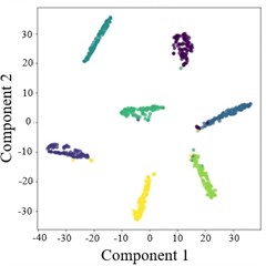
The diagnostic results of AGGCN are illustrated using the confusion matrix (Fig. 8) and the dimensionality reduction visualization (Fig. 9). As can be observed, the classification accuracy of AGGCN exhibits a clear downward trend as the noise power increases, reflecting a progressive degradation of feature separability under more severe interference. Specifically, under the noise-free setting and the 0 dB condition, the model can still capture representative fault-related patterns and maintain compact intra-class clustering with relatively large inter-class margins, thereby achieving stable and accurate recognition. However, when the noise level increases to –1 dB, –2 dB, and particularly –3 dB, the number and magnitude of non-diagonal entries in the confusion matrix increase markedly, indicating that confusion among fault categories becomes more frequent. This phenomenon is also consistent with the embedding visualization, where samples from different classes gradually overlap and the cluster boundaries become less distinct, suggesting that the learned representations are increasingly dominated by noise-induced variability rather than fault-discriminative information.

Fig. 8Confusion matrix for AGGCN cross-domain diagnosis under different noise conditions

a) Noiseless

b) 0 dB

c) –1 dB

d) –2 dB

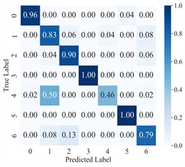
e) –3 dB

From a signal and representation learning perspective, stronger noise not only masks weak fault impulses and suppresses characteristic spectral components, but also introduces stochastic perturbations that distort temporal structures and time-frequency distributions. Consequently, the within-class variance expands while the between-class distance shrinks, which directly impairs the classifier’s ability to form robust decision boundaries. Even though AGGCN integrates time-frequency multimodal feature extraction, leverages the multiresolution and time-frequency localization properties of wavelet transforms, and benefits from the relational modeling and inherent robustness of graph convolutions, extremely strong noise can still corrupt the underlying sample correlations used to construct the graph and degrade the reliability of node/edge relationships. In other words, under high-noise regimes, both the intrinsic signal content and the cross-sample/within-sample relational cues become less trustworthy, making it increasingly challenging for the model to extract stable, condition-invariant fault features.

Nevertheless, it is noteworthy that AGGCN still achieves the best overall noise-resistance performance compared with the competing models. This advantage suggests that the proposed architecture is able to retain more informative fault cues and preserve feature structure under interference, likely due to the complementary fusion of time-frequency representations and the graph-based aggregation mechanism, which together mitigate noise sensitivity and enhance the robustness of learned diagnostic features.

Fig. 9T-SNE plots for cross-domain diagnosis of AGGCN under different noise conditions

a) Noiseless

b) 0 dB

c) –1 dB

d) –2 dB

e) –3 dB

5. Conclusions

This paper proposes a graph convolutional network GCN-based motor FD method to tackle the dual challenges posed by variable operating conditions and noise interference. Extensive comparative experiments on motor datasets demonstrate the effectiveness and robustness of the proposed approach. The main contributions and conclusions are summarized as follows:

1) A signal processing strategy that integrates time–frequency domain feature fusion and wavelet-kernel convolution is developed. Specifically, time-domain information is first extracted from raw signals via convolution and max-pooling, and then transformed into the frequency domain through FFT for further feature extraction. In addition, a wavelet-kernel convolution layer is introduced after feature fusion to initialize convolution kernels with wavelet priors, thereby strengthening the model’s capability to capture localized fault-relevant patterns and improving representation quality.

2) An attention-guided GCN-based FD framework is proposed. An attention-based graph construction mechanism is first employed to recalibrate features and efficiently generate adjacency matrices, enabling more informative and task-adaptive relational modeling. A self-loop mechanism is further incorporated to explicitly account for the contribution of each node to itself. Moreover, a multi-scale feature-fusion graph convolution layer is designed to learn diverse filtering responses across multiple branches and depths, progressively mining deeper and more discriminative fault characteristics. To accelerate convergence and enhance diagnostic accuracy, residual connections are integrated. Combined with Chebyshev graph convolutions, the framework achieves effective feature fusion over neighborhoods of different scales.

3) Experimental results on the developed test platform and relevant datasets verify that the proposed method consistently outperforms representative baseline models across multiple cross-domain tasks. On the GXU motor fault dataset, the proposed model attains an average accuracy of 95.86 % in cross-domain settings. Furthermore, it maintains strong diagnostic performance under various noise levels, demonstrating the best noise resistance among the compared approaches.

Despite these promising results, there remains room for further improvement. Future work will explore more informative feature extraction strategies to better differentiate dynamic eccentricity faults from other fault types, especially under subtle excitation conditions. In addition, given the observed performance degradation as noise intensity increases, further enhancing the model’s robustness to strong noise-potentially through more noise-aware representations, adaptive graph construction, or improved denoising mechanisms-will be an important direction for continued research.