Finite-difference analysis of seismic response in connected underground and aboveground pipelines

1. Introduction

Underground and aboveground pipelines are vital engineering structures in modern infrastructure systems. They play a key role in the uninterrupted supply of gas, water, oil and other strategic resources. However, ensuring the reliability and stability of pipeline systems in seismically active regions remains one of the pressing problems. Dynamic loads, displacements and deformations of the ground layer generated during an earthquake can lead to a sharp increase in stresses in the pipelines, damage to joints and failure of the entire system.

In recent years, a lot of scientific work has been carried out to study the dynamic state of pipeline systems under seismic impact and to develop important conclusions necessary for practice. In particular, in underground segmented pipeline systems, connecting joints are one of the weakest parts of the pipeline system, and it is in these places that the main deformation and damage occur during seismic impact [1]-[5].

Several studies have been conducted on the analytical and numerical solution of dynamic equations of underground and aboveground pipelines, in which the interaction between the pipe-soil system and the pipe and the connecting joint was obtained based on various models [6]-[11].

Although the dynamic processes in segmented underground and aboveground pipelines have been analyzed based on linear models to date, nonlinear models have not been sufficiently studied due to their complexity. In this regard, a comprehensive study of the dynamic processes of segmented underground and aboveground pipelines based on ideal elastic-plastic models is of great scientific and practical importance. Such an approach allows not only to assess the seismic resistance of the pipeline system, but also to develop optimal structural solutions and increase the level of safety. Based on these issues, the dynamic behavior of the connected segmented pipeline system for various models is analyzed theoretically and practically.

2. Material and methods

We obtain a schematic representation of a system of underground and above-ground pipelines connected by horizontally located connecting joints, as in Fig. 1.

Fig. 1Schematic view of the underground and aboveground segment piping system

a) Buried pipeline

b) Aboveground pipeline

We obtain the dynamic equation of a pipe connected by connecting joints for an ideal elastic-plastic model as follows:

Initial conditions

and the boundary conditions:

we can choose in appearance, $v_l$– speed pulse. The solution of Eq. (1-4) is presented in detail in [9], [14], [15].

To determine the deformations in the pipe and the connecting joint, we use the following relationship:

where $\epsilon$ is the pipeline strain, ${\epsilon }_s$ is the shear strain in the joint, $F_p$, $F_s$ – longitudinal force in the pipe and the connecting joint, respectively, $u_1$, $u_2$ – displacements of the left and right ends of the connecting link, respectively, $k_N$ – linear correlation coefficient, $F_{si}$, $u_{si}$ – the value of the longitudinal force and relative displacement ($u_2-u_1$) at the connecting link at this point when the process passes to the $i$-unloading state, respectively, $F_{per}$ – maximum value of longitudinal force in a nonlinear model, $l$ – the length of the pipe between two connecting joints, $A$ – cross-sectional area of a pipeline.

3. Results and discussion

Using the above materials and methods, we first analyze the dynamic processes in the above-ground pipeline based on the following values.

For the pipeline: modulus of elasticity $E=$2×10⁵MPa, density $\rho =$7800 kg/m³, each pipeline length $l=$5 m, diameter $D=$0.5 m, thickness $h=$0.01 m.

For the connecting joint: modulus of elasticity $E_S=$2·MPa, density ${\rho }_S=$930 kg/m³, length $l_S=$0.05 m, thickness $h_S=$0.01 m, linear correlation coefficient $k_N=$5.42 kN/m, limit longitudinal force $F_{per}=$4 kN.

Let us represent the velocity $v_l$ given from the left end of the pipe in the form:

where $v_0=$0.19 m/s, $T=$0.1 s, $t_0=$ 0.1 s. In general, the choice of the value of $v_0$ depends on the pipe material, tensile strength, etc. For steel pipes, the range of 0.1-3 m/s is a widely used experimental range [12], [13].

Fig. 2 shows the deformations at the joints located 5 m, 250 m and 500 m from the left end of the pipe for a period of 2 s. It can be seen from the graph that at the first joint the deformation initially reaches a maximum value and after the effect of the velocity impulse ends, the value of the deformation decreases. In this case, the maximum deformation at the joint is ${\epsilon }_{smax}=$0.074. The calculated results also show that the dynamic processes do not reach the plastic region after a distance of about 100 m and the effect of the wave decreases.

Fig. 2Deformation at connecting joints for an ideal elastic-plastic model, a – 5 m, b – 250 m, c – 500 m

In this case, the graph of deformation in the pipe will also be in the form shown in Fig. 2. In this case, the maximum deformation in the pipe is equal to ${\epsilon }_{max}=$1.37×10^–6, and the maximum value of the deformation decreases over time. It can be said that the value of the maximum deformation in the pipe is very small compared to the value of the maximum deformation in the connecting joint. The main reason for this is that a large part of the wave energy is spent on the deformation of the connecting joint, as a result of which the effect of the wave on the pipe decreases.

Now let’s look at the results of the linear model based on the above values. Fig. 3 shows the graphs of the deformations at the joints located 5 m, 250 m and 500 m from the left end of the pipe over a period of 2 s. Here, the maximum deformation at the joint is ${\epsilon }_{smax}=$0.21. From the results, it can be said that the maximum deformation at the joint calculated in the linear model is 2.83 times larger than the maximum value of the deformation calculated in the ideal elastic-plastic model.

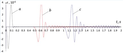
Fig. 4 shows the deformations at points in the pipe located 7.5 m, 252.5 m, and 502.5 m from the left end of the pipe over a period of 3 s. These points correspond to the midpoints of the pipe at the considered distance. In this case, the maximum deformation in the pipe is ${\epsilon }_{max}=$3.6×10^–6. In this case, the maximum deformation in the pipe calculated in the linear model is 2.63 times greater than the maximum value of the deformation calculated in the ideal elastic-plastic model.

Fig. 3Deformation at connecting joints for a linear model, a – 5 m, b – 250 m, c – 500 m

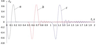
Fig. 4Deformation in the pipe for a linear model, a – 7.5 m, b – 252.5 m, c – 502.5 m

Now let us consider several dynamic cases of underground pipelines. The dynamic equations of pipes connected by joints in the ground are given in detail for a linear model [9]. Using the dynamic equations of the pipe in it, we will consider the calculated results for the ideal elastic-plastic model of the pipe and the joint. Let us take the soil with the wave propagation velocity $c=$1000 m/s and the coefficient of linear correlation of the pipe-soil system $k_x=$10⁴ kN/m³. We obtain the seismic wave velocity given in the ground in harmonic form:

where $v_{gm}=$0.19 m/s, $T=$0.33 s, $H$ – Heaviside function.

Fig. 5 shows the time-dependent deformation ${\epsilon }_s$ at the joint located 100 m from the left end of the pipe. The results are presented in the following cases: 1 – linear model, 2 – ideal elastic-plastic model, and 3 – ideal elastic-plastic model with the maximum limit longitudinal force reduced by half. Accordingly, ${\epsilon }_{s1}=$0.096, ${\epsilon }_{s2}=$0.072, ${\epsilon }_{s3}=$0.036.

Now let’s analyze the dynamic processes in the pipe.

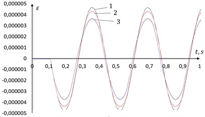
Fig. 6 shows the time-dependent deformation $\epsilon$ in the pipe located 103 m from the left end of the pipe. Here, the results are presented for the linear model 1, the ideal elastic-plastic model 2, and the ideal elastic-plastic model 3, with the maximum limiting longitudinal force reduced by half. Accordingly, ${\epsilon }_1=$4.76×10^–6, ${\epsilon }_2=$4.36×10^–6, ${\epsilon }_2=$3.69×10^–6.

It can be seen from Figs. 5-6 that the maximum deformation in long-segment underground pipes connected under the influence of seismic waves based on the ideal elastic-plastic model is several times smaller than in the linear model. It can be said that by ensuring the interaction between the connecting joint and the pipe in the form of an ideal elastic-plastic model, it is possible to prevent the occurrence of large deformations in the pipeline.

Fig. 5Deformation in the connecting joint

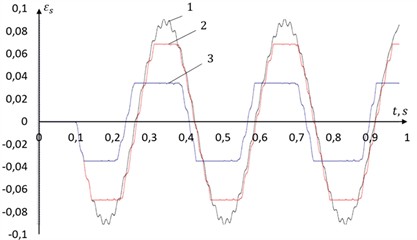
Fig. 6Deformation of underground pipeline

4. Conclusions

In this research work, the dynamic states of long underground and surface pipelines with segments connected by couplings under the influence of seismic waves were studied. When solving the dynamic equations of the pipeline, the relationship between the pipe and the couplings was taken in an ideal elastic-plastic model. When a velocity impulse is given to the surface pipelines from the left end, the largest value of the deformation is observed mainly in the area at the left end of the pipe. If the velocity impulse given from the left end of the pipe is given in a limited time interval, after the impulse effect ends, the maximum value of the deformation in the pipe and the couplings decreases over time due to the ideal elastic-plastic model. In this regard, it can be said that if the relationship between the pipe and the couplings in the design of underground and surface pipelines is chosen in the case of an ideal elastic-plastic model, the maximum value of the large stresses in the pipe and the couplings arising under the influence of seismic waves can be reduced. Based on the results obtained above and the values in the graphs, it can also be noted that if the maximum limit value of the longitudinal force in the ideal elastic-plastic model is chosen small, the maximum value of the deformation in the pipe will also decrease accordingly. This has a positive effect on preventing dangerous situations in pipelines.