Abstract
Axial crack detection in steel pipelines remains challenging because the crack-reflected guided-wave response is usually weak, frequency-dependent, and susceptible to dispersion, modal interference, sensor-coupling variation, and environmental noise. To address this issue, a reliability-adaptive probabilistic imaging and semi-quantitative severity-assessment framework is proposed using multi-frequency ultrasonic guided-wave signals. A T(0,1)-dominated torsional guided-wave packet is selected as the target response, and dispersion analysis is used to support mode selection and reflection-window prediction. Time-domain, frequency-domain, and time-frequency-domain features are extracted from the crack-reflection window to characterize the defect response from complementary perspectives. For each excitation frequency, a single-frequency probability image is constructed by combining reflected-response strength and travel-time consistency. A reliability-adaptive fusion strategy is then developed to integrate the probability images obtained at different frequencies, where the contribution of each frequency is determined by echo quality, inter-sensor consistency, and modal purity. Equal-weight fusion and SNR-weighted fusion are introduced as baseline methods to evaluate the contribution of the proposed reliability-adaptive weighting strategy. A confidence-enhancement step is further applied to suppress uncertain secondary hotspots and improve noise-interference stability under the tested controlled condition. Experiments were conducted on a Q235 steel pipe specimen containing three axial surface crack depths. The results show that amplitude- and energy-related features increase progressively with crack depth, indicating their sensitivity to severity variation under the present configuration. Compared with equal-weight and SNR-weighted fusion, the proposed method produces more compact probability distributions, lower background interference, and improved localization concentration around the actual crack region. The posterior-distribution-based severity index provides effective semi-quantitative grading of mild, moderate, and severe crack cases. The present study should be interpreted as controlled-condition verification of the proposed framework, while broader validation with different crack geometries, crack locations, sensor-coupling states, and environmental conditions is required in future work.
Highlights
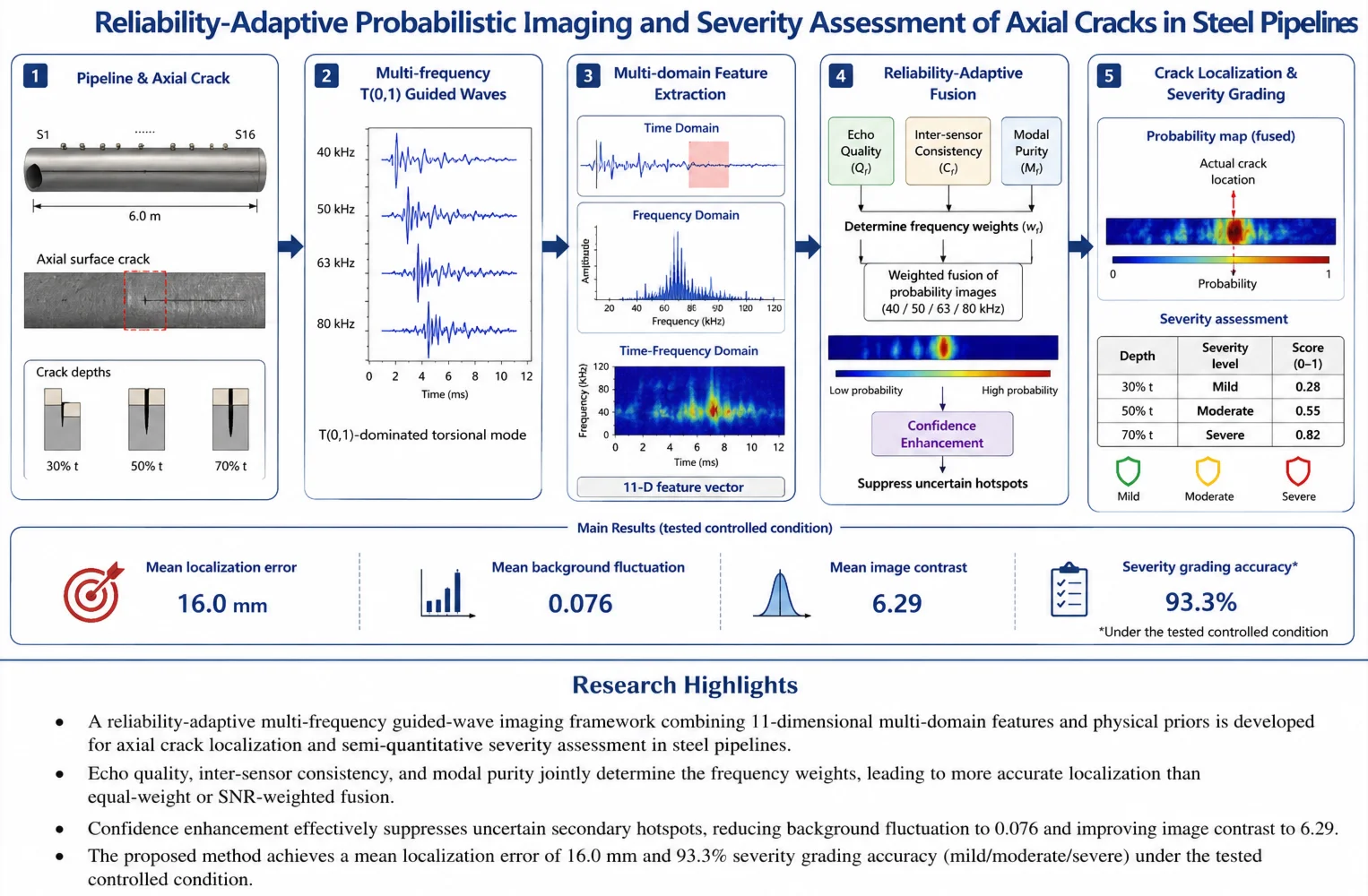
- A reliability-adaptive multi-frequency guided-wave imaging framework is developed for axial crack localization and semi-quantitative severity assessment in steel pipelines.
- Echo quality, inter-sensor consistency, and modal purity jointly determine frequency weights, improving localization compared with equal-weight and SNR-weighted fusion.
- Confidence enhancement suppresses uncertain secondary hotspots, reducing mean background fluctuation to 0.076 and increasing mean image contrast to 6.29.
- The proposed framework achieves a mean localization error of 16.0 mm and 93.3% severity-grading accuracy under the tested controlled condition.
1. Introduction
Pipelines are widely used in oil, gas, chemical, and energy transportation systems. During long-term service, internal pressure fluctuations, cyclic loading, corrosion, local stress concentration, and environmental disturbances may gradually induce wall thinning, notch-like defects, and crack-like damage. Among these defects, axial surface cracks are particularly critical because they may extend along the pipe axis and reduce the local load-bearing capacity of the pipe wall. Reliable localization and severity assessment of axial cracks are therefore important for pipeline safety evaluation, condition-based maintenance, and structural health monitoring.
Ultrasonic guided waves have been widely used for long-range pipeline inspection because they can propagate over long distances and interrogate large structural regions from a limited number of transducer locations. Rose systematically summarized the theoretical basis of ultrasonic guided waves in solid media [1], while recent reviews further confirmed their importance in nondestructive testing and structural health monitoring [2-5]. In pipe-like structures, longitudinal, torsional, and flexural guided-wave modes may coexist, and their dispersion characteristics, propagation velocities, excitation conditions, and defect sensitivities differ significantly. Therefore, inspection performance is strongly affected by mode selection, excitation frequency, sensor configuration, propagation distance, and signal-processing strategy [6-10].
Guided-wave-based pipe inspection has been studied extensively. Lowe et al. demonstrated the feasibility of pipe defect detection using guided waves [11], while Ditri investigated guided elastic waves for the characterization of circumferential cracks in hollow cylinders [12]. Focused guided waves have been used for axial crack detection in pipes [13], and the torsional T(0,1) mode has been investigated for circumferential and longitudinal defect detection because of its relatively stable propagation behavior in suitable frequency ranges [14]. Crack characterization using guided circumferential waves has also been reported [16], and the excitation of guided elastic wave modes in hollow cylinders has been analyzed from the viewpoint of applied surface tractions [17]. These studies provide an important physical basis for pipe guided-wave inspection, but they also show that the measured defect response depends strongly on guided-wave mode, frequency, propagation path, and defect geometry.
Axial crack detection remains challenging because the crack-reflected wave packet is usually weak and may be contaminated by multimodal propagation, pipe-end reflections, dispersion, coupling variation, and environmental noise. Dispersion effects are especially important in long-range guided-wave inspection because they can broaden the received wave packet and reduce the accuracy of arrival-time interpretation [9], [10]. Wavelet analysis and other time-frequency signal-processing methods have therefore been introduced to improve the interpretation of guided-wave responses in pipe inspection [19]. In addition, matching-pursuit-based signal characterization has been used to extract defect-related information from guided-wave signals [29]. Although these methods improve signal interpretation, a single waveform feature or a single excitation frequency is often insufficient for stable axial-crack localization and severity assessment.
Guided-wave imaging aims to convert scattered-wave information into spatially interpretable damage maps. Hayashi and Murase demonstrated defect imaging with guided waves in pipes [15], and subsequent studies showed that crack-like defects, notches, holes, bends, coatings, buried conditions, and corrosion profiles may all influence the guided-wave response and the corresponding image interpretation [18], [23-30]. In the broader field of guided-wave structural health monitoring, probability-based imaging, RAPID-type diagnostic imaging, delay-and-sum imaging, tomographic reconstruction, and fusion-based imaging strategies are commonly used to transform path-dependent guided-wave measurements into damage probability maps. These methods provide intuitive localization results, but their performance may be affected by sparse sensor layouts, velocity errors, modal interference, predefined spatial influence functions, and the unequal quality of signals obtained at different frequencies or channels. For pipeline inspection, these issues are particularly important because the pipe geometry, guided-wave dispersion, modal conversion, and boundary reflections can jointly affect the reliability of reconstructed images.
Multi-frequency guided-wave testing can provide complementary information for crack detection. Low-frequency excitation usually offers better propagation stability and lower attenuation, whereas higher-frequency excitation may improve local defect sensitivity and spatial resolution. However, higher frequencies may also introduce stronger dispersion, modal interference, and noise-interference sensitivity [9], [10]. The excitation and propagation of the torsional T(0,1) mode have been widely investigated for pipeline integrity testing [20-22], and scattering from crack-like defects in hollow cylinders has also been analyzed [23]. These studies support the use of a T(0,1)-dominated torsional guided-wave response for pipeline defect inspection. Nevertheless, different excitation frequencies do not necessarily provide the same level of measurement reliability. Equal-weight fusion may therefore introduce weak or noisy frequency components into the final image. Existing fusion concepts, including Bayesian fusion, evidence-theory-based fusion, signal-to-noise-ratio-based weighting, feature-level fusion, and decision-level fusion, provide useful ideas for combining heterogeneous information. However, in practical guided-wave pipeline inspection, a physically interpretable fusion strategy should consider not only echo amplitude or noise level, but also inter-sensor consistency and modal purity.
Crack severity assessment is another important issue in guided-wave-based pipeline inspection. Existing severity-related approaches can be broadly divided into four categories. The first category uses amplitude-, energy-, or reflection-coefficient-based indicators, which are physically intuitive because deeper or larger defects generally produce stronger guided-wave scattering and reflection responses [18], [30]. However, these indicators are sensitive to propagation distance, sensor coupling, attenuation, and excitation frequency. The second category extracts signal features from the reflected wave packet, such as time-domain, frequency-domain, time-frequency-domain, or sparse-representation features, to improve the description of defect-induced waveform changes [19], [29]. These feature-based methods provide richer information than a single amplitude metric, but their performance may still fluctuate when modal interference or noise is significant. The third category is model-based or inverse reconstruction, in which crack size or depth is estimated by matching measured responses with forward scattering models. Such methods may provide more direct quantitative interpretation, but they usually require accurate material parameters, boundary conditions, defect geometry assumptions, and sufficient measurement paths. The fourth category uses data-driven regression or classification models. For example, convolutional neural networks have recently been used for quantitative detection of pipeline cracks based on ultrasonic guided waves [31]. Nevertheless, machine-learning-based methods generally require representative training datasets covering different crack locations, sizes, sensor-coupling states, and environmental variations.
Therefore, in the present controlled experiment, the proposed severity assessment is positioned as a semi-quantitative grading strategy rather than an absolute crack-depth inversion method. Instead of relying only on reflected amplitude, reflected energy, or a single machine-learning output, this study constructs a posterior-distribution-based severity index from the confidence-enhanced probability image. This design allows crack severity to be evaluated from local posterior intensity, regional probability distribution, high-response area, and cross-frequency consistency.
Based on the above discussion, three main gaps remain. First, existing guided-wave imaging studies provide useful localization strategies, but the unequal reliability of different excitation frequencies is not always explicitly considered in the imaging process. Second, multi-frequency guided-wave responses are affected by echo quality, inter-sensor consistency, and modal purity, but these factors are not always incorporated into a unified and physically interpretable fusion measure. Third, crack severity assessment is often treated separately from probabilistic imaging, and the severity-related information contained in the posterior probability distribution has not been sufficiently utilized.
To address these issues, this study proposes a reliability-adaptive probabilistic imaging and severity-assessment framework for axial surface cracks in steel pipelines using multi-frequency ultrasonic guided-wave signals. The novelty of this work does not lie in proposing a completely new guided-wave imaging theory. Instead, the contribution lies in integrating frequency-dependent probabilistic indications, measurement-reliability weighting, confidence-enhanced probability mapping, and posterior-distribution-based severity grading into a unified framework under a controlled pipeline inspection configuration.
The main contributions of this study are summarized as follows. First, a multi-domain guided-wave feature representation is constructed from the crack-reflection window by combining time-domain, frequency-domain, and time-frequency-domain descriptors. Second, a single-frequency probabilistic imaging formulation is established by combining reflected-response strength and travel-time consistency on the imaging grid. Third, a reliability-adaptive multi-frequency fusion strategy is developed using echo quality, inter-sensor consistency, and modal purity, so that the contribution of each frequency is determined by measurement reliability rather than by equal weighting. Fourth, a confidence-enhanced probabilistic imaging step is introduced to suppress uncertain secondary hotspots. Finally, a posterior-distribution-based severity index is proposed for semi-quantitative grading of mild, moderate, and severe axial crack cases.
The experimental validation is conducted on one Q235 steel pipe specimen containing one intact case and three axial surface crack cases with different depths. The crack location, length, width, and orientation are fixed, and repeated measurements are used mainly to evaluate repeatability and noise-interference sensitivity rather than to represent independent crack configurations. Therefore, the present results should be interpreted as controlled-condition verification of the proposed framework. Broader validation involving different crack positions, crack lengths, crack widths, crack orientations, sensor-coupling conditions, and environmental disturbances will be required in future work.
The remainder of this paper is organized as follows. Section 2 describes the experimental setup, guided-wave mode selection, dispersion analysis, and signal preprocessing procedure. Section 3 presents the proposed probabilistic imaging, reliability-adaptive fusion, confidence enhancement, and severity-assessment methods. Section 4 discusses the experimental results, baseline comparison, ablation analysis, and limitations. Section 5 summarizes the main conclusions.
2. Experimental setup and guided-wave mode analysis
2.1. Steel pipeline specimen and damage scenarios
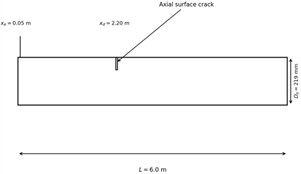
A straight Q235 steel pipeline specimen was used to evaluate the proposed reliability-adaptive probabilistic imaging and severity-assessment framework under controlled laboratory conditions. The specimen had an outer diameter of 219 mm, a wall thickness of 5 mm, an inner diameter of 209 mm, and a total length of 6.0 m. The material parameters used in the analysis were Young’s modulus 206 GPa, Poisson’s ratio 0.30, and mass density 7850 kg/m3. The specimen geometry and crack arrangement are shown in Fig. 1, and the corresponding geometric and material parameters are summarized in Table 1.
Table 1Geometric and material parameters of the steel pipeline specimen
Parameter | Symbol | Value | Unit |
Pipe length | 6.0 | m | |
Outer diameter | 219 | mm | |
Inner diameter | 209 | mm | |
Wall thickness | 5 | mm | |
Young’s modulus | 206 | GPa | |
Poisson’s ratio | 0.30 | – | |
Density | 7850 | kg/m3 | |
Excitation axial position | 0.05 | m | |
Crack axial position | 2.20 | m | |
Crack circumferential position | 180 | deg |
One intact case, denoted as N0, and three damaged cases, denoted as C1-C3, were considered. The damaged cases were machined as external axial rectangular notches on the outer surface of the pipe. In all damaged cases, the axial location, circumferential location, crack length, and crack width were kept unchanged, while only the crack depth was varied. This controlled design was adopted to isolate the influence of crack depth on the guided-wave response. Therefore, the present experiment should be interpreted as a controlled-condition verification rather than a full generalization to arbitrary crack geometries, crack orientations, or pipe environments.
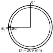
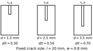
The crack length and width were fixed at 20 mm and 0.8 mm, respectively. The crack center was located at 2.20 m and 180°. The relative crack depth was defined as , where is the notch depth and is the pipe wall thickness. The three damaged cases corresponded to depth ratios of 0.30, 0.50, and 0.70, representing mild, moderate, and severe axial surface cracks, respectively. The detailed definitions of the damage cases are listed in Table 2.
Fig. 1Geometry of the steel pipeline specimen and crack configuration: a) overall geometry of the Q235 steel pipeline specimen; b) pipe cross-section and crack circumferential position; c) definitions of the three crack-depth cases C1, C2, and C3
a)
b)
c)
Table 2Definition of damage cases and severity levels
Case | Condition | Crack length () / mm | Crack width () / mm | Crack depth () / mm | Depth ratio () | Severity label |
N0 | Intact pipe | 0 | 0 | 0 | 0 | None |
C1 | Axial surface crack | 20 | 0.8 | 1.5 | 0.30 | Mild |
C2 | Axial surface crack | 20 | 0.8 | 2.5 | 0.50 | Moderate |
C3 | Axial surface crack | 20 | 0.8 | 3.5 | 0.70 | Severe |
2.2. Measurement setup, excitation configuration, and sensor arrangement
The guided-wave measurement system was configured to capture the incident wave packet, the crack-reflected response, and the subsequent boundary-related echoes. The actuator position, receiver layout, excitation waveform, and acquisition parameters were kept unchanged for all intact and damaged cases to ensure that the measured differences were mainly caused by crack-depth variation. Since guided-wave measurements in pipes are sensitive to transducer configuration, modal content, sensor spacing, and coupling conditions [6], [10], [13], these experimental parameters were controlled throughout the tests.
The axial coordinate was defined from the left end of the pipe, and the circumferential coordinate was measured from the reference generatrix of the pipe. The excitation transducer was mounted on the outer surface of the pipe at 0.05 m. Sixteen receiving sensors were arranged along the same circumferential side as the crack to improve the sensitivity to the back-scattered crack response. The receiver positions were = 0.40, 0.80, 1.20, 1.60, 2.00, 2.40, 2.80, 3.20, 3.60, 4.00, 4.40, 4.80, 5.20, 5.40, 5.60, and 5.80 m, corresponding to channels S1-S16, respectively. Channels S5-S8 were located closest to the crack region and were selected as the principal observation channels for representative signal and feature analysis, while all available receiving channels were used in the imaging and fusion procedure.
A five-cycle Hanning-windowed sinusoidal burst was used as the excitation signal. Four center frequencies, namely 40, 50, 63, and 80 kHz, were adopted to investigate the frequency dependence of the crack-reflected response and to provide the basis for multi-frequency fusion. This low-frequency guided-wave range provides a practical compromise among propagation attenuation, spatial resolution, and modal complexity in pipeline inspection [14], [20-22]. The excitation voltage was fixed at 100 V for all test conditions. The signals received were sampled at 10 MHz with a record length of 12 ms, which was sufficient to cover the incident wave, the crack-reflected component, and later reflections from pipe boundaries.
The excitation configuration was designed to obtain a torsional-mode-dominated guided-wave response in the selected low-frequency range. In the revised manuscript, this response is referred to as the T(0,1)-dominated wave packet rather than an ideally pure single-mode wave, because weak residual modal components may still exist in practical measurements. The dominance of the target wave packet was verified by comparing the measured arrival time with the group velocity predicted from the dispersion analysis in Section 2.3. This cautious description avoids overclaiming pure single-mode excitation while still clarifying the dominant mode used for reflection-window prediction and probabilistic imaging.
Each measurement condition was repeated 20 times. These repeated measurements were used to evaluate signal repeatability, noise-interference sensitivity, and the stability of extracted features. They were not treated as independent pipe specimens or independent crack configurations. The sensor layout is illustrated in Fig. 2, and the detailed acquisition parameters are listed in Table 3.
Fig. 2Guided-wave measurement setup and layout of the actuator and receiving sensors
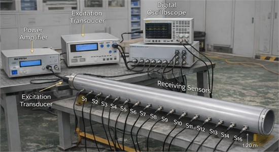
Table 3Experimental parameters for guided-wave excitation and signal acquisition
Parameter | Symbol | Value | Unit |
Excitation waveform | – | 5-cycle Hanning-windowed sinusoidal burst | – |
Excitation frequencies | 40, 50, 63, 80 | kHz | |
Target dominant mode | – | T(0,1)-dominated torsional wave packet | – |
Excitation voltage | 100 | V | |
Excitation axial position | 0.05 | m | |
Sampling frequency | 10 | MHz | |
Record length | 12 | ms | |
Number of receiving channels | 16 | – | |
Number of repeated measurements | 20 | – | |
Group velocity used for window prediction | Approximately 3260 | m/s | |
Main analysis channels | – | S5–S8 | – |
2.3. Guided-wave mode selection and dispersion analysis
Guided waves in cylindrical structures generally contain longitudinal, torsional, and flexural modes. These modes have different propagation velocities, dispersion characteristics, and sensitivity to defect orientation. Therefore, the target wave mode should be clarified before reflection-window extraction and probabilistic imaging. In this study, the T(0,1)-dominated torsional guided-wave response was selected as the target wave packet for subsequent analysis.
The selection of the T(0,1)-dominated response was based on two considerations. First, the torsional T(0,1) mode is nearly non-dispersive in the investigated low-frequency range, which is beneficial for predicting the arrival time of the crack-reflected wave packet [1], [14], [17], [20]. Second, the relatively stable group velocity of the torsional response reduces the uncertainty caused by frequency-dependent wave-packet spreading. This property is important for multi-frequency feature extraction and probabilistic imaging because the same physical reflection event must be isolated consistently at different excitation frequencies.
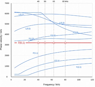
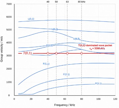
To verify the selected mode and the group velocity used in this study, a dispersion analysis was performed for the Q235 steel pipe using the geometric and material parameters listed in Table 1. The calculated phase-velocity and group-velocity curves are shown in Fig. 3. The four excitation frequencies used in the experiment, namely 40, 50, 63, and 80 kHz, are marked on the dispersion curves. In this frequency range, the selected T(0,1)-dominated response shows a group velocity close to 3260 m/s. Therefore, 3260 m/s was used for theoretical prediction of the crack-reflection arrival time.
The addition of dispersion analysis also addresses the reproducibility of the experimental configuration. Recent guided-wave studies on complex pipe-like structures have similarly used phase- and group-velocity dispersion curves to guide mode selection and inspection-parameter design [32]. In the present study, the dispersion result provides the physical basis for both the reflection-window calculation and the later reliability-adaptive fusion strategy. Although the same target wave packet is considered at all excitation frequencies, the received signal quality, modal purity, and scattering sensitivity may still vary with frequency. Therefore, the later fusion procedure does not assign equal importance to all frequencies but determines their relative contributions according to measurement reliability.
Fig. 3Dispersion curves and mode selection for the Q235 steel pipe: a) phase-velocity dispersion curves; b) group-velocity dispersion curves. The four excitation frequencies of 40, 50, 63, and 80 kHz are marked, and the selected T(0,1)-dominated wave packet shows a group velocity close to in the investigated frequency range
a)
b)
2.4. Signal preprocessing and reflection-window extraction
The raw guided-wave measurements contained the incident wave packet, crack-reflected components, pipe-end reflections, residual modal components, and broadband environmental noise. Since the crack-reflected response was much weaker than the directly transmitted wave packet, signal preprocessing was required before feature extraction and probabilistic imaging. The preprocessing procedure included direct-current removal, amplitude normalization, narrow-band filtering, and wavelet denoising. Signal-processing strategies such as multimode signal interpretation, dispersion-related analysis, filtering, and wavelet-based denoising have been widely used to improve the interpretability of guided-wave measurements [8-10], [19].
Let denote the raw signal measured at receiver i, excitation frequency f, and repeated measurement m. After direct-current removal and amplitude normalization, the normalized signal was obtained as:
where denotes the mean value of the raw signal over the full record, and the denominator denotes the maximum absolute amplitude of the zero-mean signal. This normalization constrains the full-record amplitude to the range of [–1, 1], thereby reducing amplitude fluctuations caused by channel sensitivity and repeated-measurement variation. Accordingly, the revised signal-preprocessing figure should use a normalized-amplitude axis covering [–1, 1]. If a local reflection segment is enlarged for clarity, it should be explicitly labelled as a zoomed view.
After normalization, a zero-phase band-pass filter centered at the excitation frequency was used to suppress out-of-band noise and non-target components. Wavelet denoising was then applied to further improve the signal-to-noise ratio of the crack-related response while preserving the main waveform characteristics. The preprocessing parameters for different excitation frequencies are summarized in Table 4.
The crack-related information was mainly concentrated in the reflected wave packet. Therefore, a dedicated reflection window was extracted from each preprocessed signal. The expected arrival time of the crack-reflected wave was estimated from the actuator-crack-receiver propagation path as:
where is the propagation distance from the actuator to the crack, is the propagation distance from the crack to receiver , and is the group velocity of the selected T(0,1)-dominated wave packet at frequency f. In the present frequency range, was approximately 3260 m/s, as indicated by the dispersion analysis in Section 2.3.
A time window centered at was then extracted for each channel and frequency. The crack-reflected signal segment was defined as:
where is the window length used at frequency . A frequency-dependent window length was adopted to account for the different wave-packet durations at different excitation frequencies. The window was selected to include the main crack-reflected packet while reducing the influence of pipe-end echoes and non-target wave components.
A representative example of the preprocessing and reflection-window extraction is shown in Fig. 4. The full-record signal is displayed using the normalized-amplitude range of [–1, 1], while the extracted crack-reflection segment is presented as a zoomed view to better illustrate the local waveform characteristics around the expected reflection time. This representation allows the overall signal evolution and the weak crack-reflected wave packet to be observed simultaneously.
The resulting reflection-window signals were used for subsequent time-domain, frequency-domain, and time-frequency-domain feature extraction. By combining mode-guided arrival-time prediction, amplitude-normalized preprocessing, and frequency-dependent reflection-window extraction, the weak crack-reflected response could be isolated more consistently from the complex guided-wave background.
Fig. 4Example of signal preprocessing and reflection-window extraction for C2 at 50 kHz in channel S6: a) raw full-record signal after normalization, with the normalized amplitude displayed in the range of [–1,1]; b) preprocessed signal after band-pass filtering and wavelet denoising, with the reflection window highlighted. (c) Zoomed view of the extracted crack-reflected wave packet
![Example of signal preprocessing and reflection-window extraction for C2 at 50 kHz in channel S6: a) raw full-record signal after normalization, with the normalized amplitude displayed in the range of [–1,1]; b) preprocessed signal after band-pass filtering and wavelet denoising, with the reflection window highlighted. (c) Zoomed view of the extracted crack-reflected wave packet](https://static-01.extrica.com/articles/26338/26338-img7.jpg)
a)
![Example of signal preprocessing and reflection-window extraction for C2 at 50 kHz in channel S6: a) raw full-record signal after normalization, with the normalized amplitude displayed in the range of [–1,1]; b) preprocessed signal after band-pass filtering and wavelet denoising, with the reflection window highlighted. (c) Zoomed view of the extracted crack-reflected wave packet](https://static-01.extrica.com/articles/26338/26338-img8.jpg)
b)
![Example of signal preprocessing and reflection-window extraction for C2 at 50 kHz in channel S6: a) raw full-record signal after normalization, with the normalized amplitude displayed in the range of [–1,1]; b) preprocessed signal after band-pass filtering and wavelet denoising, with the reflection window highlighted. (c) Zoomed view of the extracted crack-reflected wave packet](https://static-01.extrica.com/articles/26338/26338-img9.jpg)
c)
Table 4Signal preprocessing settings for different excitation frequencies
Frequency / kHz | Filter band / kHz | Wavelet basis | Decomposition level | Reflection-window length / ms |
40 | 30–50 | db4 | 4 | 1.2 |
50 | 40–60 | db4 | 4 | 1.0 |
63 | 53–73 | db4 | 5 | 0.9 |
80 | 70–90 | db4 | 5 | 0.8 |
3. Proposed reliability-adaptive probabilistic imaging framework
3.1. Overall processing flow
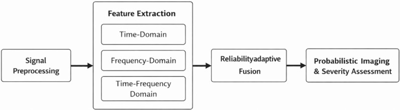
The proposed framework transforms the measured guided-wave responses into probabilistic crack-localization images and semi-quantitative severity-grading results. As shown in Fig. 5, the procedure consists of six main steps: reflection-window signal extraction, multi-domain feature extraction, single-frequency probabilistic imaging, reliability-adaptive multi-frequency fusion, confidence-enhanced probabilistic imaging, and posterior-distribution-based severity assessment.
After preprocessing and reflection-window extraction, each receiver channel and excitation frequency provides a crack-related signal segment. Time-domain, frequency-domain, and time-frequency-domain descriptors are then extracted from this segment to characterize the crack-reflected response from complementary perspectives. For each excitation frequency, a single-frequency probability field is constructed on the imaging grid by combining reflection intensity and travel-time consistency. The probability fields obtained at different frequencies are then fused using reliability-adaptive weights. These weights are determined by echo quality, inter-sensor consistency, and modal purity, so that frequency components with higher measurement reliability contribute more strongly to the final image.
This design follows the general guided-wave inspection logic in which signal preprocessing, modal interpretation, feature extraction, and spatial imaging are combined to improve defect detectability in pipe-like structures [2-4], [15], [29], [31]. After multi-frequency fusion, a confidence-enhancement step is introduced to suppress uncertain secondary hotspots in the probability field. Finally, several posterior-distribution features are extracted from the confidence-enhanced image and combined into a severity index for semi-quantitative grading. Compared with direct equal-weight fusion, the proposed framework emphasizes the reliability and physical consistency of the measured information rather than treating all frequencies and channels as equally informative.
Fig. 5Overall processing flow of the proposed reliability-adaptive probabilistic imaging and severity-assessment framework
3.2. Multi-domain feature extraction
Guided-wave crack responses may exhibit changes in amplitude, energy, arrival time, spectral distribution, and local time-frequency concentration. Such multi-domain signal variations are closely related to multimodal propagation, dispersion, defect scattering, and time-frequency characteristics of guided-wave measurements [8-10], [18], [19]. A single descriptor is therefore insufficient to represent the weak and frequency-dependent crack-reflected response. For this reason, a multi-domain feature vector was constructed from the reflection-window signal.
Let denote the extracted crack-reflected signal segment measured at receiver , excitation frequency , and repeated measurement , where is the discrete sampling time and . The reflected peak amplitude is defined as:
The reflected energy is calculated as:
where is the sampling interval. The peak-based arrival time of the reflected wave packet is defined as:
where is the start time of the extracted reflection window. The arival-time descriptor is mainly used to evaluate whether the measured crack-related response is consistent with the theoretical actuator-crack-receiver propagation path.
Frequency-domain and time-frequency-domain descriptors were introduced because defect scattering may redistribute signal energy in the spectrum and produce localized time-frequency variations that are not fully captured by time-domain peak features alone [18], [19], [29]. Let be the amplitude spectrum of the reflection-window signal at frequency bin . The dominant frequency is defined as:
and the spectral centroid is defined as:
To further describe the local time-frequency organization of the crack response, a time-frequency representation was computed using a short-time or wavelet-based time-frequency transform. The total time-frequency energy is given by:
The time-frequency concentration factor is defined as:
where is a small positive constant used to avoid division by zero. A larger TFC value indicates that the crack-related energy is concentrated in a more compact time-frequency region.
The extracted descriptors were stacked into a multi-domain feature vector:
Table 5Extracted multi-domain features used for crack characterization
Feature | Symbol | Domain | Physical interpretation |
Reflected peak amplitude | Time domain | Maximum amplitude of the crack-reflected wave packet | |
Reflected energy | Time domain | Total energy of the crack-reflected wave packet | |
Peak arrival time | Time domain | Travel-time consistency of the reflected response | |
Dominant frequency | Frequency domain | Spectral peak position of the reflected response | |
Spectral centroid | Frequency domain | Global spectral balance of the reflected response | |
Time-frequency energy | Time-frequency domain | Total local energy in the time-frequency plane | |
Time-frequency concentration factor | TFC | Time-frequency domain | Compactness of crack-related time-frequency energy |
Multi-domain feature vector | Integrated | Unified representation for imaging and fusion |
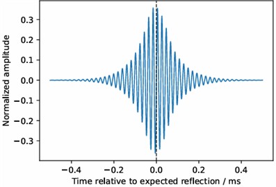
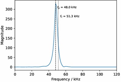
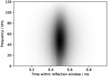
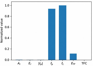
Before probabilistic imaging and fusion, each feature component was standardized to zero mean and unit variance across the corresponding dataset. This normalization prevents features with large numerical scales from dominating the subsequent analysis. The adopted multi-domain feature descriptors are summarized in Table 5, and a representative feature-extraction example is illustrated in Fig. 6.
Fig. 6Example of multi-domain feature extraction from the crack-reflected wave packet
a)
b)
c)
d)
3.3. Single-frequency probabilistic imaging formulation
To clarify the generation of the frequency-specific probability field, an imaging grid was defined in the axial-circumferential plane of the pipe. Each candidate pixel is denoted by . For a given excitation frequency , the theoretical arrival time of a crack-reflected wave associated with receiver and candidate position is expressed as:
where is the propagation distance from the actuator to the candidate pixel, is the propagation distance from the candidate pixel to receiver and is the group velocity of the selected T(0,1)-dominated wave packet at frequency . This path-consistency concept is consistent with guided-wave imaging studies in which candidate damage locations are evaluated according to the agreement between measured wave arrivals and theoretically predicted propagation paths [13], [15], [18].
The travel-time consistency between the measured response and the candidate pixel is evaluated by:
where is the measured peak arrival time and controls the tolerance of arrival-time deviation. A larger value of indicates that the candidate pixel is more consistent with the measured reflection arrival time.
The response strength of each receiver channel is described by a normalized damage-sensitive feature score:
where the tilde denotes normalized feature values. The coefficients - are non-negative and satisfy:
In this study, the same feature-score definition was used for all frequencies to avoid frequency-specific manual tuning.
The single-frequency probabilistic indication is then calculated as:
where is the number of receiving channels used for imaging. The normalized single-frequency probability field is obtained by:
Thus, , and a larger value indicates a stronger probability that the candidate pixel corresponds to the crack-related reflection source. This formulation links the probability image to both reflected-response strength and travel-time consistency, rather than generating the image only from empirical visual smoothing.
3.4. Reliability-adaptive multi-frequency fusion
The single-frequency probability fields may differ significantly because guided-wave scattering, modal purity, signal-to-noise ratio, and sensor consistency vary with excitation frequency. Previous studies on torsional guided-wave excitation and pipeline defect interaction have shown that the received response may vary with excitation frequency, modal condition, propagation path, and defect geometry [14], [20-23]. Equal-weight fusion assumes that all frequencies are equally reliable, which may introduce unstable or weakly informative frequency components into the final image. To address this issue, a reliability-adaptive fusion strategy was used to combine the probability fields obtained at different excitation frequencies.
Let be the single-frequency probability field at frequency . The fused probability field is defined as:
where 40, 50, 63, 80 kHz is the set of excitation frequencies, and is the weight assigned to frequency . The weights satisfy:
To evaluate the contribution of the proposed weighting strategy, two baseline fusion strategies were also considered. The first baseline is equal-weight fusion, in which all excitation frequencies are assigned the same contribution, i.e., , where is the number of excitation frequencies. This strategy is simple and commonly used as a direct baseline, but it assumes that all frequency components have identical reliability.
The second baseline is SNR-weighted fusion. In this baseline, the contribution of each frequency is determined only by the echo-to-noise level, i.e., , where denotes the echo-quality indicator defined below. This baseline is used to examine whether considering noise level alone is sufficient for multi-frequency fusion. Compared with equal-weight fusion, SNR-weighted fusion can suppress frequencies with weak crack-related echoes or high pre-reflection noise. However, it does not explicitly consider whether the defect-sensitive response is spatially consistent among sensors or whether the reflected wave packet is dominated by the target guided-wave mode.
In the proposed reliability-adaptive fusion strategy, three measurement-oriented reliability indicators were used to determine : echo quality, inter-sensor consistency, and modal purity. The echo-quality indicator is defined as:
where is the mean reflected peak amplitude over the selected receiver channels and repeated measurements, and is the standard deviation of the pre-reflection noise at frequency . A larger indicates a stronger crack-related echo relative to background noise.
The inter-sensor consistency indicator is defined as:
where denotes the coefficient of variation. This term assigns a larger value to a frequency whose damage-sensitive responses are more consistent across receiver channels.
The modal-purity indicator is defined as:
where is the energy contained in the target modal band around the selected T(0,1)-dominated wave packet, and is the total energy in the reflection window. This term penalizes frequency components with stronger non-target modal contamination.
The adaptive weight is calculated by multiplicative normalization:
where , , and control the relative importance of echo quality, inter-sensor consistency, and modal purity, respectively. Unless otherwise stated, was used to avoid over-parameterization. In this way, a frequency receives a large contribution only when it simultaneously exhibits strong echo quality, stable inter-sensor response, and acceptable modal purity.
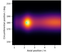
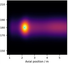
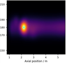
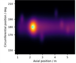
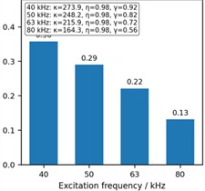
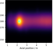
Compared with equal-weight fusion and SNR-weighted fusion, Eq. (23) incorporates three physically interpretable reliability factors. Therefore, the proposed fusion strategy is better described as a reliability-informed multi-frequency integration mechanism rather than a purely empirical weighting scheme. A representative example of the single-frequency probability images, adaptive weights, and fused probability image is shown in Fig. 7.
Fig. 7Reliability-adaptive multi-frequency fusion results for the representative case of C2: a)-d) show the single-frequency probabilistic images reconstructed at 40, 50, 63, and 80 kHz, respectively; e) presents the adaptive weights determined by echo quality, inter-sensor consistency, and modal purity; f) shows the fused probability image obtained by reliability-adaptive multi-frequency fusion
a)
b)
c)

d)
e)
f)
3.5. Confidence-enhanced probabilistic imaging
Although reliability-adaptive fusion improves the utilization of frequency-dependent information, the fused image may still contain secondary hotspots when several non-damage regions exhibit moderate probability. To suppress uncertain indications without excessively smoothing the dominant crack response, a confidence-enhancement step was introduced after multi-frequency fusion.
For each candidate pixel , the uncertainty of the fused probability field is quantified using binary entropy:
The corresponding confidence coefficient is defined as:
The confidence-enhanced probability image is then obtained as:
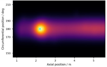
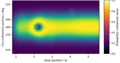
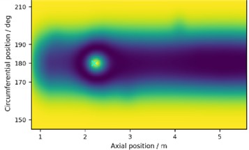
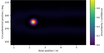
According to Eqs. (24-26), pixels with high fused probability and low uncertainty are retained, whereas pixels with moderate but ambiguous probability are attenuated. This operation is used as an uncertainty-control step rather than a purely visual image-sharpening procedure. The posterior uncertainty, confidence coefficient, and confidence-enhanced probability image are illustrated in Fig. 8.
Fig. 8Illustration of posterior uncertainty and confidence-enhanced imaging for the representative case of C2: a) shows the fused probability image; b) shows the posterior uncertainty distribution; c) shows the confidence coefficient distribution; d) shows the confidence-enhanced probability image
a)
b)
c)
d)
3.6. Severity index for crack assessment
Before defining the proposed severity index, it is necessary to clarify its relationship with existing severity-assessment indicators. In guided-wave inspection, reflected peak amplitude, reflected energy, and reflection-coefficient-related quantities are commonly used to describe defect severity because they are directly associated with defect-induced scattering strength [18], [30]. Feature-based methods further incorporate waveform, spectral, or time-frequency descriptors to improve sensitivity to damage-related signal variations [19], [29]. However, these conventional indicators are usually extracted from individual signals or selected channels, and they may be affected by sensor coupling, propagation distance, noise level, and frequency-dependent modal behavior. In contrast, the severity index used in this study is extracted from the posterior probability image after reliability-adaptive multi-frequency fusion and confidence enhancement. Therefore, it does not replace physical amplitude or energy indicators, but integrates them into a spatial probabilistic representation for semi-quantitative crack grading.
The final objective of the proposed framework is not only to localize the crack but also to provide a semi-quantitative assessment of crack severity. Since reflected amplitude, reflected energy, and extracted signal features are commonly used to describe defect-induced guided-wave scattering, the severity index in this study is constructed from posterior-distribution features rather than from a single waveform descriptor [18], [29], [30]. This design allows the severity assessment to consider peak posterior intensity, regional response level, high-probability spatial extent, and cross-frequency stability.
The crack candidate location is first determined by:
A region of interest is then defined around . The peak posterior response is:
The regional mean response is calculated as:
The high-response area is defined as:
where is the indicator function, is the relative high-response threshold, and is the area represented by one imaging pixel.
The cross-frequency consistency is defined as:
This term evaluates whether different excitation frequencies provide consistent evidence at the estimated crack location.
Before constructing the severity index, , , , were normalized to the range of [0, 1]. The overall severity index is defined as:
where:
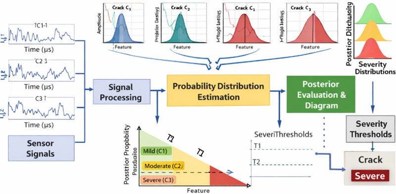
In the present controlled experiment, the weighting coefficients were selected to balance local posterior intensity, regional distribution, high-response extent, and cross-frequency stability. The influence of these coefficients is further discussed in the ablation and limitation analysis in Section 4.6. The damage grade is finally determined by two thresholds and :
It should be emphasized that the proposed index is designed for semi-quantitative severity grading rather than absolute crack-depth inversion. The thresholds and are calibrated under the present controlled experimental configuration and should be recalibrated when additional crack geometries, locations, orientations, or sensor-coupling conditions are introduced. The complete severity-grading procedure based on posterior distribution features is summarized in Fig. 9.
Fig. 9Flowchart of crack severity grading based on posterior distribution features
4. Results and discussion
4.1. Response of multi-domain features to crack severity
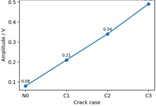
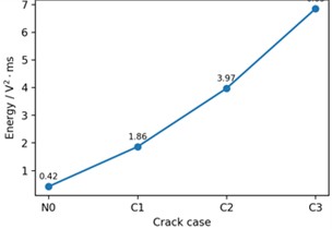
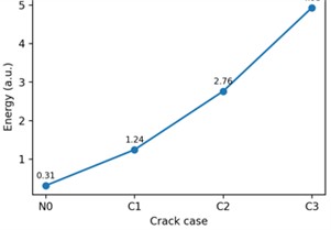
The response of representative multi-domain features to crack severity is shown in Fig. 10 and summarized in Table 6. Under the present controlled experimental configuration, the reflected peak amplitude , reflected energy , and time-frequency energy increased progressively from the intact case N0 to the severe crack case C3. This trend indicates that deeper axial surface notches produced stronger back-scattered guided-wave responses and higher local time-frequency energy. Such amplitude- and energy-related variations are consistent with the general physical interpretation of guided-wave scattering from notch-like defects [18], [19], [29].
By contrast, the peak arrival time changed only slightly among C1-C3. This is expected because the crack location was fixed in all damaged cases, and the dominant actuator-crack-receiver propagation path remained unchanged. Therefore, in the present experiment, the arrival-time descriptor mainly supports localization consistency rather than severity discrimination. This also confirms the necessity of using different descriptors for different assessment purposes: arrival-time information is more relevant to spatial localization, whereas amplitude- and energy-related features are more sensitive to crack-depth variation.
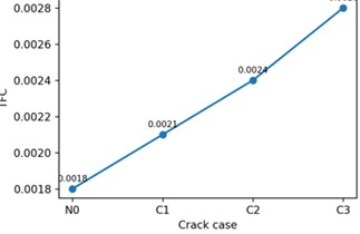
The frequency-domain descriptors showed a relatively moderate trend. The dominant frequency and spectral centroid varied within a narrow range, suggesting that crack deepening did not fundamentally shift the central frequency content of the reflected wave packet. However, the increase in and TFC indicates that the crack-related energy became more concentrated as the crack depth increased. These observations support the use of a multi-domain feature vector rather than a single waveform descriptor.
It should be noted that the observed monotonic trends were obtained with a fixed crack position, fixed crack length, fixed crack width, and fixed crack orientation. Therefore, the feature response should be interpreted as depth-sensitive behavior under controlled conditions, rather than as a complete representation of all possible axial crack configurations.
Fig. 10Comparison of representative multi-domain features under different crack conditions: a)-d) show the variations of the reflected peak amplitude, reflected energy, time-frequency energy, and time-frequency concentration factor TFC, respectively, for the intact case N0 and the three crack cases C1-C3
a)
b)
c)
d)
Table 6Statistical values of representative multi-domain features for different damage cases
Case | / V | / a.u. | / ms | / kHz | / kHz | / a.u. | TFC |
N0 | 0.08 | 0.42 | 6.31 | 49.8 | 50.6 | 0.35 | 0.214 |
C1 | 0.21 | 1.86 | 6.34 | 50.3 | 51.2 | 1.42 | 0.287 |
C2 | 0.34 | 3.97 | 6.36 | 50.7 | 52.1 | 2.88 | 0.351 |
C3 | 0.49 | 6.85 | 6.39 | 51.1 | 53.4 | 4.76 | 0.426 |
4.2. Single-frequency probabilistic imaging and frequency dependence
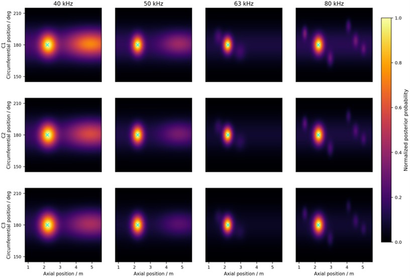
Fig. 11 compares the single-frequency probabilistic images obtained at 40, 50, 63, and 80 kHz for the three damaged cases C1-C3. All four excitation frequencies produced a damage-sensitive indication in the vicinity of the actual crack position, indicating that each frequency retained a certain degree of axial-crack sensitivity. However, the compactness of the hotspot, the level of background response, and the stability of localization differed among the four frequencies.
The 40 kHz results generally produced broader probability distributions. This behavior can be explained by the relatively longer wavelength and lower spatial resolution at lower frequency. Although the low-frequency response is usually more stable for long-distance propagation, its ability to concentrate the probability field around a small crack region is limited. The 80 kHz results showed stronger local sensitivity in some cases, but they were also more susceptible to background fluctuation and possible modal interference. This is consistent with the frequency-dependent nature of guided-wave propagation and scattering in pipe-like structures [14], [20-23].
For the present specimen and crack configuration, 50 and 63 kHz provided a better balance between crack-response strength, localization compactness, and background suppression. Nevertheless, the results also show that no single frequency was uniformly optimal for all crack depths. A frequency that provides a clear response for a severe crack may not necessarily provide the most stable response for a mild crack. Therefore, relying on a fixed single-frequency inspection strategy may lead to inconsistent imaging quality when the crack severity is unknown.
These single-frequency results provide the experimental motivation for multi-frequency fusion. The purpose of fusion is not simply to accumulate all available frequency responses, but to integrate complementary information while suppressing frequency components with lower measurement reliability.
Fig. 11Single-frequency probabilistic imaging results at 40, 50, 63, and 80 kHz for axial crack cases C1-C3. The actual crack position is marked in each image
4.3. Comparison with equal-weight and SNR-weighted fusion
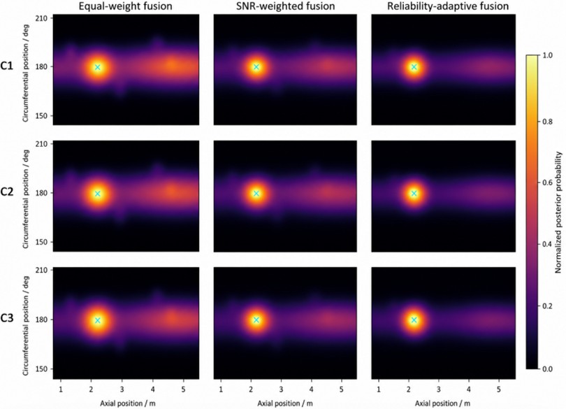
Fig. 12 and Table 7 compare three multi-frequency fusion strategies: equal-weight fusion, SNR-weighted fusion, and the proposed reliability-adaptive fusion. The equal-weight fusion method assigns identical contributions to all excitation frequencies, whereas the SNR-weighted baseline determines the frequency weights only from the echo-to-noise level. The proposed method further incorporates inter-sensor consistency and modal purity in addition to echo quality.
All three methods produced damage-sensitive indications near the actual crack region, indicating that multi-frequency combination is beneficial compared with relying on a single frequency alone. However, the equal-weight fusion images showed broader high-probability regions and stronger background artifacts, especially for the mild and moderate crack cases. This behavior is expected because all frequency components contribute identically even when their echo quality, modal purity, or inter-sensor consistency is relatively poor.
The SNR-weighted fusion baseline reduced part of the background response because frequency components with lower echo-to-noise levels were assigned smaller weights. For example, the localization error decreased from 42 mm to 30 mm for C1, from 35 mm to 25 mm for C2, and from 27 mm to 18 mm for C3. The background fluctuation also decreased compared with equal-weight fusion. Nevertheless, some secondary probability distributions remained because SNR weighting does not explicitly evaluate whether the defect-sensitive response is spatially consistent among sensors or whether the reflected wave packet is dominated by the target guided-wave mode.
Compared with both baselines, the proposed reliability-adaptive fusion produced more concentrated probability distributions around the actual crack position. For C1, the localization error decreased from 42 mm using equal-weight fusion and 30 mm using SNR-weighted fusion to 21 mm using the proposed method. For C2, the localization error decreased from 35 mm and 25 mm to 16 mm. For C3, it decreased from 27 mm and 18 mm to 11 mm. The high-response area and background fluctuation were also reduced, while the image contrast increased. These results indicate that the proposed weighting strategy improves localization concentration not simply by amplifying high-SNR frequency components, but by suppressing frequency components with poor echo quality, unstable inter-sensor response, or stronger non-target modal contamination.
Although the present comparison is still limited to fusion-based baselines and does not include RAPID-type probability imaging, delay-and-sum imaging, or tomographic reconstruction, the addition of the SNR-weighted baseline provides a more direct evaluation of the methodological contribution of the proposed reliability-adaptive weighting strategy.
Fig. 12Comparison of equal-weight fusion, SNR-weighted fusion, and reliability-adaptive fusion imaging results for C1-C3. The left column shows equal-weight fusion, the middle column shows SNR-weighted fusion, and the right column shows reliability-adaptive fusion. The actual crack position is marked in each image
4.4. Confidence-enhanced imaging under noise interference
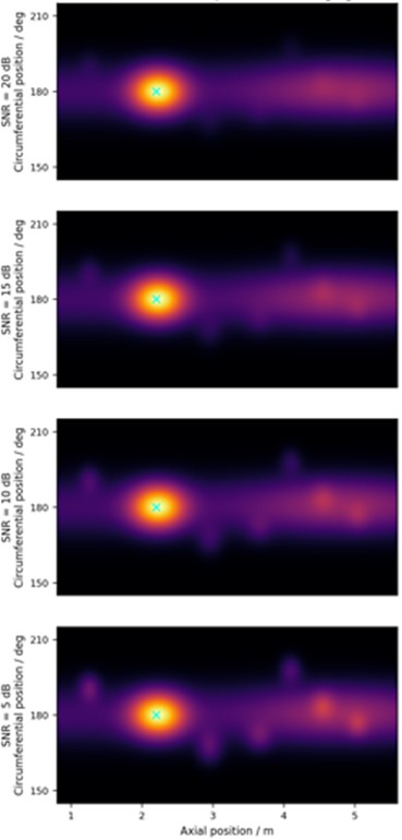
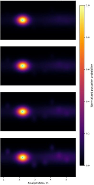
The effect of the confidence-enhancement step was examined under different noise levels. As shown in Fig. 13, the rows correspond to SNR levels of 20, 15, 10, and 5 dB, while the left and right columns represent the conventional probabilistic images and the confidence-enhanced results, respectively. The quantitative comparison is summarized in Table 8.
Table 7Quantitative comparison of localization and imaging performance for different fusion strategies
Damage case | Fusion strategy | Peak response | Localization error / mm | High-response area / pixels | Background fluctuation | Image contrast |
C1 | Equal-weight fusion | 0.71 | 42 | 1860 | 0.184 | 3.26 |
C1 | SNR-weighted fusion | 0.78 | 30 | 1520 | 0.147 | 4.12 |
C1 | Reliability-adaptive fusion | 0.83 | 21 | 1240 | 0.117 | 4.82 |
C2 | Equal-weight fusion | 0.79 | 35 | 2145 | 0.173 | 3.74 |
C2 | SNR-weighted fusion | 0.85 | 25 | 1727 | 0.134 | 4.66 |
C2 | Reliability-adaptive fusion | 0.89 | 16 | 1385 | 0.102 | 5.41 |
C3 | Equal-weight fusion | 0.86 | 27 | 2480 | 0.161 | 4.18 |
C3 | SNR-weighted fusion | 0.90 | 18 | 1952 | 0.123 | 5.16 |
C3 | Reliability-adaptive fusion | 0.94 | 11 | 1520 | 0.091 | 5.96 |
As the SNR decreased, the conventional fused probability images exhibited more secondary hotspots and stronger background fluctuations. This behavior is expected because random noise and unstable wave-packet fluctuations can produce moderate probability values at non-damage locations. When the confidence coefficient defined in Eq. (25) was applied, these uncertain responses were attenuated, while the dominant crack-related indication remained visible.
Table 8Quantitative comparison of conventional fusion and confidence-enhanced imaging under different noise levels
SNR / dB | Method | Peak response | False-hotspot number | Background fluctuation | Mean confidence coefficient | Image contrast |
20 | Conventional fusion | 0.88 | 2 | 0.096 | 0.742 | 5.38 |
20 | Confidence-enhanced imaging | 0.86 | 1 | 0.071 | 0.814 | 6.27 |
15 | Conventional fusion | 0.84 | 4 | 0.128 | 0.693 | 4.61 |
15 | Confidence-enhanced imaging | 0.82 | 2 | 0.089 | 0.781 | 5.74 |
10 | Conventional fusion | 0.79 | 7 | 0.173 | 0.621 | 3.92 |
10 | Confidence-enhanced imaging | 0.77 | 3 | 0.108 | 0.736 | 5.03 |
5 | Conventional fusion | 0.71 | 11 | 0.241 | 0.548 | 3.11 |
5 | Confidence-enhanced imaging | 0.69 | 5 | 0.139 | 0.684 | 4.26 |
The improvement became more obvious under lower SNR conditions. At 20 dB, the false-hotspot number decreased from 2 to 1, and the image contrast increased from 5.38 to 6.27. At 5 dB, the false-hotspot number decreased from 11 to 5, and the background fluctuation decreased from 0.241 to 0.139. These results indicate that the confidence-enhancement step is especially useful when the probability field contains competing uncertain regions.
It should be emphasized that the confidence-enhancement step is not intended to create new crack information. Instead, it acts as an uncertainty-control operation applied to the fused probability field. Regions with high probability and low uncertainty are retained, whereas regions with moderate and ambiguous probability are suppressed. Therefore, the observed improvement should be interpreted as improved noise-interference stability under the tested controlled condition, rather than as general robustness against arbitrary pipeline environments.
Fig. 13Comparison of conventional probabilistic imaging and confidence-enhanced imaging under different noise levels. Rows correspond to SNR levels of 20, 15, 10, and 5 dB. The left column shows conventional probabilistic imaging, whereas the right column shows the corresponding confidence-enhanced results
a) Conventional probabilistic imaging
b) Confidence-enhanced imaging
4.5. Severity grading performance
The severity index defined in Eqs. (27-34) was evaluated for the three axial crack depths. As shown in Fig. 14, the severity index increased progressively from C1 to C3. Fig. 15 further shows that the three crack cases could be separated into mild, moderate, and severe regions using the calibrated thresholds. The corresponding severity-related posterior features, including , , , , and the final severity index , are listed in Table 9, and the confusion matrix is summarized in Table 10.
For comparison with conventional severity-assessment logic, the proposed severity index should be interpreted against three typical benchmark indicators: reflected peak amplitude, reflected energy, and peak posterior probability. Reflected peak amplitude and reflected energy provide direct descriptions of scattering strength, and their monotonic increase from C1 to C3 confirms that the measured guided-wave response is sensitive to crack-depth variation under the present controlled configuration. However, these two indicators are single-signal or feature-level quantities and do not directly describe whether the corresponding response is spatially concentrated around the actual crack position. The peak posterior probability provides a spatially interpretable indicator, but it may still be insufficient when two cases have similar peak values but different high-response areas or frequency consistency. The proposed severity index combines peak posterior response, regional mean probability, high-response area, and cross-frequency consistency; therefore, it provides a more comprehensive benchmark for semi-quantitative grading than a single amplitude-, energy-, or peak-probability-based criterion.
Fig. 14Distribution of the proposed severity index for different crack cases
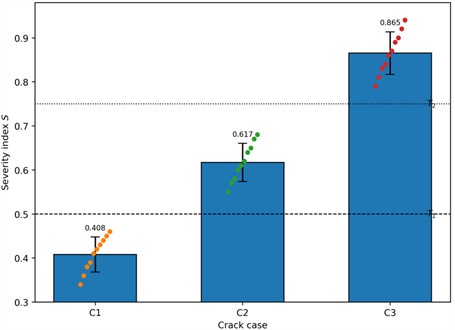
Fig. 15Grading results of mild, moderate, and severe cracks based on the proposed severity index
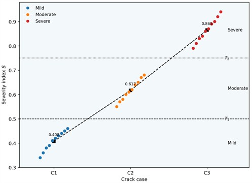
The grading results indicate that the confidence-enhanced probability image contains severity-related distributional information under the present controlled configuration. Mild cracks produced lower peak response and smaller high-response area, whereas severe cracks produced stronger local probability and a larger consistent high-response region. This suggests that crack severity is reflected not only in the maximum probability value, but also in the spatial distribution of the posterior field.
The proposed severity index is therefore more informative than a simple peak-value criterion for the tested cases. By combining , , , , the index considers local intensity, regional distribution, spatial extent, and cross-frequency consistency. This posterior-distribution-based design provides a semi-quantitative grading indicator under the present controlled experimental condition, but it should not be interpreted as a general crack-depth inversion model.
Table 9Severity-related indicators and final grading results for different crack cases
Case | / pixels | Severity index () | Grading result | |||
C1 | 0.78 | 0.42 | 865 | 0.81 | 0.56 | Mild |
C2 | 0.87 | 0.55 | 1240 | 0.86 | 0.71 | Moderate |
C3 | 0.94 | 0.68 | 1635 | 0.91 | 0.84 | Severe |
Table 10Confusion matrix and grading accuracy of the proposed crack severity assessment method
Actual class | Predicted as mild | Predicted as moderate | Predicted as severe | Classification accuracy / % |
Mild (C1) | 10 | 0 | 0 | 100.0 |
Moderate (C2) | 1 | 9 | 0 | 90.0 |
Severe (C3) | 0 | 1 | 9 | 90.0 |
Overall accuracy: 93.3 % | ||||
The confusion matrix shows an overall grading accuracy of 93.3 % for the tested repeated measurements. Nevertheless, this value should be interpreted carefully. The repeated measurements were obtained from the same pipe specimen and the same crack geometry, and they should not be regarded as independent specimens. Therefore, the grading result demonstrates repeatability under the present controlled configuration rather than general classification capability across arbitrary crack locations, lengths, widths, orientations, or sensor-coupling conditions.
4.6. Ablation and limitation analysis
To further clarify the contribution of different components in the proposed framework, an ablation comparison was conducted based on the quantitative results of multi-frequency fusion, confidence-enhanced imaging, and severity grading. The analysis focused on three key components that can be evaluated from the present experimental results: SNR-weighted fusion, reliability-adaptive weighting, and confidence enhancement. The mean localization error, mean high-response area, mean background fluctuation, and mean image contrast were calculated by averaging the results over the three crack cases C1-C3.
The equal-weight fusion result was used as the basic baseline. The SNR-weighted fusion baseline was introduced to evaluate whether echo-to-noise information alone is sufficient for frequency weighting. The contribution of reliability-adaptive weighting was evaluated by comparing the SNR-weighted baseline and the proposed reliability-adaptive fusion. The contribution of confidence enhancement was estimated using the 20 dB noise condition as the representative low-noise case, because this condition is closest to the original experimental measurement state. The severity accuracy was obtained from the final grading confusion matrix. The corresponding ablation results are summarized in Table 11.
As shown in Table 11, the equal-weight baseline produced a mean localization error of 34.67 mm, a mean high-response area of 2161.67 pixels, a mean background fluctuation of 0.173, and a mean image contrast of 3.73. After SNR-weighted fusion was introduced, the mean localization error decreased to 24.33 mm, the mean high-response area decreased to 1733.00 pixels, the mean background fluctuation decreased to 0.135, and the mean image contrast increased to 4.65. This confirms that echo-to-noise information is useful for suppressing weak or noisy frequency components.
However, SNR-weighted fusion was still inferior to the proposed reliability-adaptive fusion. When inter-sensor consistency and modal purity were further incorporated into the weighting strategy, the mean localization error decreased to 16.00 mm, the mean high-response area decreased to 1381.67 pixels, the mean background fluctuation decreased to 0.103, and the mean image contrast increased to 5.40. These results indicate that the improvement of the proposed method is not caused only by higher echo amplitude or lower noise level. Instead, the additional use of response consistency and modal-purity information helps suppress frequency components that are not physically reliable for crack localization.
Table 11Ablation comparison of different framework components under the controlled experimental configuration
Method | Feature set | Fusion strategy | Confidence enhancement | Mean localization error / mm | Mean high-response area / pixels | Mean background fluctuation | Mean image contrast | Severity accuracy / % |
Equal-weight baseline | Multi-domain | Equal-weight | No | 34.67 | 2161.67 | 0.173 | 3.73 | – |
SNR-weighted baseline | Multi-domain | SNR-weighted | No | 24.33 | 1733.00 | 0.135 | 4.65 | – |
Without adaptive weighting | Multi-domain | Equal-weight | Yes | 34.67 | 2161.67 | 0.128 | 4.34 | – |
Without confidence enhancement | Multi-domain | Reliability-adaptive | No | 16.00 | 1381.67 | 0.103 | 5.40 | – |
Proposed framework | Multi-domain | Reliability-adaptive | Yes | 16.00 | 1381.67 | 0.076 | 6.29 | 93.3 |
The confidence-enhancement step further reduced background fluctuation and improved image contrast. When confidence enhancement was applied to the equal-weight baseline, the mean background fluctuation decreased from 0.173 to 0.128, and the mean image contrast increased from 3.73 to 4.34. When it was applied after reliability-adaptive fusion, the mean background fluctuation decreased from 0.103 to 0.076, and the mean image contrast increased from 5.40 to 6.29. These results show that confidence enhancement mainly acts as an uncertainty-control step for reducing ambiguous secondary probability regions, rather than as an independent source of crack information.
The proposed framework achieved a severity grading accuracy of 93.3 % for the tested repeated measurements. This result suggests that the confidence-enhanced posterior probability distribution contains useful severity-related information under the present controlled configuration. Nevertheless, this value should not be interpreted as general classification performance for arbitrary pipeline defects. The repeated measurements were obtained from the same pipe specimen and the same crack geometry, and they were used mainly to evaluate repeatability and noise-interference stability under the tested controlled condition. Broader validation with different crack positions, crack lengths, crack widths, crack orientations, sensor-coupling states, and environmental conditions is still required.
The present comparison is also limited in terms of baseline methods. Although equal-weight fusion and SNR-weighted fusion provide two useful fusion-based baselines, additional comparisons with RAPID-type probability imaging, delay-and-sum imaging, tomographic reconstruction, and data-driven regression methods should be conducted in future work when comparable sensor-network configurations and datasets are available. Therefore, the present results should be regarded as controlled-condition verification of the proposed reliability-adaptive probabilistic imaging and semi-quantitative severity-assessment framework.
5. Conclusions
This study proposed a reliability-adaptive probabilistic imaging and semi-quantitative severity-assessment framework for axial surface cracks in steel pipelines using multi-frequency ultrasonic guided-wave signals. A T(0,1)-dominated torsional guided-wave packet was selected as the target response, and dispersion analysis was introduced to support guided-wave mode selection and reflection-window prediction. Based on the extracted crack-reflected wave packet, time-domain, frequency-domain, and time-frequency-domain features were constructed to describe the defect response from complementary perspectives.
The experimental results obtained from the Q235 steel pipe specimen show that amplitude- and energy-related features increase progressively from the mild crack case to the severe crack case. This indicates that the extracted multi-domain features are sensitive to crack-depth variation under the present controlled configuration. The arrival-time-related descriptor showed only limited variation among the three crack cases because the crack location was fixed, confirming that arrival-time information is more suitable for localization consistency than for severity discrimination in this experiment.
A reliability-adaptive multi-frequency fusion strategy was developed by combining echo quality, inter-sensor consistency, and modal purity. Compared with equal-weight fusion and SNR-weighted fusion, the proposed fusion strategy produced more concentrated probability distributions around the actual crack region, reduced background fluctuation, and improved image contrast. These results indicate that considering noise level alone is insufficient for multi-frequency guided-wave imaging, and that response consistency and modal purity are also important for selecting reliable frequency components.
The confidence-enhancement step further suppressed uncertain secondary hotspots in the fused probability image. Its main function is not to generate additional crack information, but to attenuate ambiguous probability regions with higher uncertainty. Therefore, the observed improvement should be interpreted as enhanced noise-interference stability under the tested controlled condition, rather than as general robustness for arbitrary pipeline environments.
A posterior-distribution-based severity index was constructed using the peak posterior response, regional mean probability, high-response area, and cross-frequency consistency. The grading results show that the proposed index can distinguish mild, moderate, and severe axial crack cases under the present experimental configuration. Compared with single amplitude-, energy-, or peak-probability-based indicators, the proposed index provides a more comprehensive semi-quantitative description by combining local intensity, spatial distribution, high-response extent, and frequency consistency.
It should be emphasized that the present validation was conducted on one straight Q235 steel pipe specimen with a fixed crack location, length, width, and orientation, while only the crack depth was varied. The repeated measurements were used mainly to evaluate repeatability and noise-interference stability under the tested controlled condition, and should not be regarded as independent crack configurations. Therefore, the results should be interpreted as controlled-condition verification of the proposed framework rather than full validation for arbitrary pipeline crack scenarios. Future work will include different crack positions, crack lengths, crack widths, crack orientations, sensor-coupling states, pipe boundary conditions, and environmental disturbances. Additional comparisons with RAPID-type probability imaging, delay-and-sum imaging, tomographic reconstruction, and data-driven regression methods will also be conducted to further evaluate the generalization capability of the proposed method.
References
-
J. L. Rose, Ultrasonic Guided Waves in Solid Media. Cambridge, United Kingdom: Cambridge University Press, 2014, https://doi.org/10.1017/cbo9781107273610
-
P. Cawley, “Guided waves in long range nondestructive testing and structural health monitoring: principles, history of applications and prospects,” NDT and E International, Vol. 142, p. 103026, 2024, https://doi.org/10.1016/j.ndteint.2023.103026
-
X. Zang, Z.-D. Xu, H. Lu, C. Zhu, and Z. Zhang, “Ultrasonic guided wave techniques and applications in pipeline defect detection: a review,” International Journal of Pressure Vessels and Piping, Vol. 206, p. 105033, Jul. 2023, https://doi.org/10.1016/j.ijpvp.2023.105033
-
Z. Yang et al., “A review on guided-ultrasonic-wave-based structural health monitoring: from fundamental theory to machine learning techniques,” Ultrasonics, Vol. 133, p. 107014, Apr. 2023, https://doi.org/10.1016/j.ultras.2023.107014
-
F. Lyu, X. Zhou, Z. Ding, X. Qiao, and D. Song, “Application research of ultrasonic-guided wave technology in pipeline corrosion defect detection: a review,” Coatings, Vol. 14, No. 3, p. 358, Mar. 2024, https://doi.org/10.3390/coatings14030358
-
H. Miao and F. Li, “Shear horizontal wave transducers for structural health monitoring and nondestructive testing: a review,” Ultrasonics, Vol. 114, p. 106355, Feb. 2021, https://doi.org/10.1016/j.ultras.2021.106355
-
D. N. Alleyne and P. Cawley, “The interaction of Lamb waves with defects,” IEEE Transactions on Ultrasonics, Ferroelectrics and Frequency Control, Vol. 39, No. 3, pp. 381–397, 1992, https://doi.org/10.1109/58.143172
-
D. Alleyne and P. Cawley, “A two-dimensional Fourier transform method for the measurement of propagating multimode signals,” The Journal of the Acoustical Society of America, Vol. 89, No. 3, pp. 1159–1168, Mar. 1991, https://doi.org/10.1121/1.400530
-
P. Wilcox, M. Lowe, and P. Cawley, “The effect of dispersion on long-range inspection using ultrasonic guided waves,” NDT and E International, Vol. 34, No. 1, pp. 1–9, 2001, https://doi.org/10.1016/s0963-8695(00)00024-4
-
P. D. Wilcox, “A rapid signal processing technique to remove the effect of dispersion from guided wave signals,” IEEE Transactions on Ultrasonics, Ferroelectrics and Frequency Control, Vol. 50, No. 4, pp. 419–427, 2003, https://doi.org/10.1109/tuffc.2003.1197965
-
M. J. S. Lowe, D. N. Alleyne, and P. Cawley, “Defect detection in pipes using guided waves,” Ultrasonics, Vol. 36, No. 1-5, pp. 147–154, Apr. 2003, https://doi.org/10.1016/s0041-624x(97)00038-3
-
J. J. Ditri, “Utilization of guided elastic waves for the characterization of circumferential cracks in hollow cylinders,” The Journal of the Acoustical Society of America, Vol. 96, No. 6, pp. 3769–3775, Dec. 1994, https://doi.org/10.1121/1.410565
-
S. Fletcher, M. J. S. Lowe, M. Ratassepp, and C. Brett, “Detection of axial cracks in pipes using focused guided waves,” Journal of Nondestructive Evaluation, Vol. 31, No. 1, pp. 56–64, Nov. 2011, https://doi.org/10.1007/s10921-011-0120-x
-
Z. Liu, C. He, B. Wu, X. Wang, and S. Yang, “Circumferential and longitudinal defect detection using T(0,1) mode excited by thickness shear mode piezoelectric elements,” Ultrasonics, Vol. 44, No. 1, pp. e1135–e1138, Jun. 2006, https://doi.org/10.1016/j.ultras.2006.05.154
-
T. Hayashi and M. Murase, “Defect imaging with guided waves in a pipe,” The Journal of the Acoustical Society of America, Vol. 117, No. 4, pp. 2134–2140, Apr. 2005, https://doi.org/10.1121/1.1862572
-
C. Valle, M. Niethammer, J. Qu, and L. J. Jacobs, “Crack characterization using guided circumferential waves,” The Journal of the Acoustical Society of America, Vol. 110, No. 3, pp. 1282–1290, Sep. 2001, https://doi.org/10.1121/1.1385899
-
J. J. Ditri and J. L. Rose, “Excitation of guided elastic wave modes in hollow cylinders by applied surface tractions,” Journal of Applied Physics, Vol. 72, No. 7, pp. 2589–2597, Oct. 1992, https://doi.org/10.1063/1.351558
-
A. Demma, P. Cawley, M. Lowe, A. G. Roosenbrand, and B. Pavlakovic, “The reflection of guided waves from notches in pipes: a guide for interpreting corrosion measurements,” NDT and E International, Vol. 37, No. 3, pp. 167–180, 2004, https://doi.org/10.1016/j.ndteint.2003.09.004
-
M. H. S. Siqueira, C. E. N. Gatts, R. R. Da Silva, and J. M. A. Rebello, “The use of ultrasonic guided waves and wavelets analysis in pipe inspection,” Ultrasonics, Vol. 41, No. 10, pp. 785–797, Feb. 2004, https://doi.org/10.1016/j.ultras.2004.02.013
-
X. Niu, W. Duan, H.-P. Chen, and H. R. Marques, “Excitation and propagation of torsional T(0,1) mode for guided wave testing of pipeline integrity,” Measurement, Vol. 131, pp. 341–348, Aug. 2018, https://doi.org/10.1016/j.measurement.2018.08.021
-
X. Niu, K. F. Tee, and H. R. Marques, “Enhancement of unidirectional excitation of guided torsional T(0,1) mode by linear superposition of multiple rings of transducers,” Applied Acoustics, Vol. 168, p. 107411, May 2020, https://doi.org/10.1016/j.apacoust.2020.107411
-
Z. Fan, X. Niu, B. Miao, and H. Meng, “Hybrid coded excitation of the torsional guided wave mode T(0,1) for oil and gas pipeline inspection,” Applied Sciences, Vol. 12, No. 2, p. 777, Jan. 2022, https://doi.org/10.3390/app12020777
-
X. Zhang, Z. Tang, F. Lv, and K. Yang, “Scattering of torsional flexural guided waves from circular holes and crack-like defects in hollow cylinders,” NDT and E International, Vol. 89, pp. 56–66, 2017, https://doi.org/10.1016/j.ndteint.2017.03.007
-
S. Heinlein, P. Cawley, and T. K. Vogt, “Reflection of torsional T(0,1) guided waves from defects in pipe bends,” NDT and E International, Vol. 93, pp. 57–63, 2018, https://doi.org/10.1016/j.ndteint.2017.09.007
-
M. Qi, S. Zhou, J. Ni, and Y. Li, “Investigation on ultrasonic guided waves propagation in elbow pipe,” International Journal of Pressure Vessels and Piping, Vol. 139-140, pp. 250–255, Feb. 2016, https://doi.org/10.1016/j.ijpvp.2016.02.026
-
B. Verma, T. K. Mishra, K. Balasubramaniam, and P. Rajagopal, “Interaction of low-frequency axisymmetric ultrasonic guided waves with bends in pipes of arbitrary bend angle and general bend radius,” Ultrasonics, Vol. 54, No. 3, pp. 801–808, Oct. 2013, https://doi.org/10.1016/j.ultras.2013.10.007
-
E. Leinov, M. J. S. Lowe, and P. Cawley, “Investigation of guided wave propagation and attenuation in pipe buried in sand,” Journal of Sound and Vibration, Vol. 347, pp. 96–114, Mar. 2015, https://doi.org/10.1016/j.jsv.2015.02.036
-
A. C. Cobb, H. Kwun, L. Caseres, and G. Janega, “Torsional guided wave attenuation in piping from coating, temperature, and large-area corrosion,” NDT and E International, Vol. 47, pp. 163–170, 2012, https://doi.org/10.1016/j.ndteint.2012.01.002
-
P. W. Tse and X. Wang, “Characterization of pipeline defect in guided-waves based inspection through matching pursuit with the optimized dictionary,” NDT and E International, Vol. 54, pp. 171–182, 2013, https://doi.org/10.1016/j.ndteint.2012.10.003
-
R. Carandente, A. Lovstad, and P. Cawley, “The influence of sharp edges in corrosion profiles on the reflection of guided waves,” NDT and E International, Vol. 52, pp. 57–68, 2012, https://doi.org/10.1016/j.ndteint.2012.08.008
-
Y. Shen, J. Wu, J. Chen, W. Zhang, X. Yang, and H. Ma, “Quantitative detection of pipeline cracks based on ultrasonic guided waves and convolutional neural network,” Sensors, Vol. 24, No. 4, p. 1204, Feb. 2024, https://doi.org/10.3390/s24041204
-
X. Wan, S. Ma, H. Pan, X. Zhang, L. Huang, and Y. Chen, “Non-disassembled inspection of drill pipe threaded connections via ultrasonic guided waves,” Engineering Structures, Vol. 357, p. 122563, Mar. 2026, https://doi.org/10.1016/j.engstruct.2026.122563
-
X. Wan, S. Chen, L. Huang, X. Zhang, X. Cao, and Y. Chen, “Review on static component generation of ultrasonic waves in solid media,” AIP Advances, Vol. 15, No. 6, p. 060702, Jun. 2025, https://doi.org/10.1063/5.0243601
About this article

This work was supported by the Inner Mongolia Natural Science Foundation, China, under Grant No. 2024LHMS06004 (2024-2026), entitled “Research on High-Order Helical Guided Wave Detection and Visualization Methods for Defects in Hydrogen Storage Cylinder Containers”, and by the Graduate Scientific Research and Innovation Project of the Education Department of Inner Mongolia Autonomous Region under Grant No. KC2025064S. This work was supported by the Open Project Program of the State Key Laboratory of Special Vehicle Design and Manufacturing Integration Technology under Grant No. GZ2025KF001.
The datasets generated during and/or analyzed during the current study are available from the corresponding author on reasonable request.
Changzhi He: conceptualization, methodology, software, investigation, formal analysis, visualization, writing-original draft preparation. Xinyu Zhang: supervision, funding acquisition, project administration, methodology, validation, writing-review and editing. Zhen Li: resources, validation, formal analysis, writing-review and editing.
The authors declare that they have no conflict of interest.

