Numerical analysis of vortex-induced flow structures and their spectral characteristics behind a square cylinder using adaptive and locally refined grids

Madaliev, Murodil; Mamurov, Eldor; Tadjibayev, Rasul; Gaynazarov, Abdulvasiy; Mamirov, Abdurashid; Nishonova, Gazaloy

doi:10.21595/vp.2026.26474

Vibroengineering Procedia

Browse Procedia

Published: July 16, 2026

Check for updates

Numerical analysis of vortex-induced flow structures and their spectral characteristics behind a square cylinder using adaptive and locally refined grids

Murodil Madaliev¹

Eldor Mamurov²

Rasul Tadjibayev³

Abdulvasiy Gaynazarov⁴

Abdurashid Mamirov⁵

Gazaloy Nishonova⁶

^{1, 2, 3, 4, 5, 6}Fergana State Technical University, Fergana, Uzbekistan

Corresponding Author:

Murodil Madaliev

Cite the article Download PDF

Downloads 22

Abstract

In this paper, the vortex flow structures formed behind a square cylinder and their spectral properties are numerically investigated based on the 2D URANS $k$ - $ω$ SST model (Re ≈ 4.7×10⁴). The study compared locally densified and adaptive anisotropic (Hessian-based) meshes. The calculations were performed using the PISO algorithm and second-order accuracy (CFL ≤ 1, $Δ t \approx T$ /200). The results were compared with experimental data on Strouhal number, drag and lift coefficients, and velocity profiles. The adaptive mesh more accurately represents the wake zone and sharp gradients of the flow, allows for reliable estimation of spectral parameters (frequency and amplitude), and reduces numerical diffusion. Some limitations of the 2D URANS model are also indicated.

Numerical analysis of vortex-induced flow structures and their spectral characteristics behind a square cylinder using adaptive and locally refined grids

Highlights

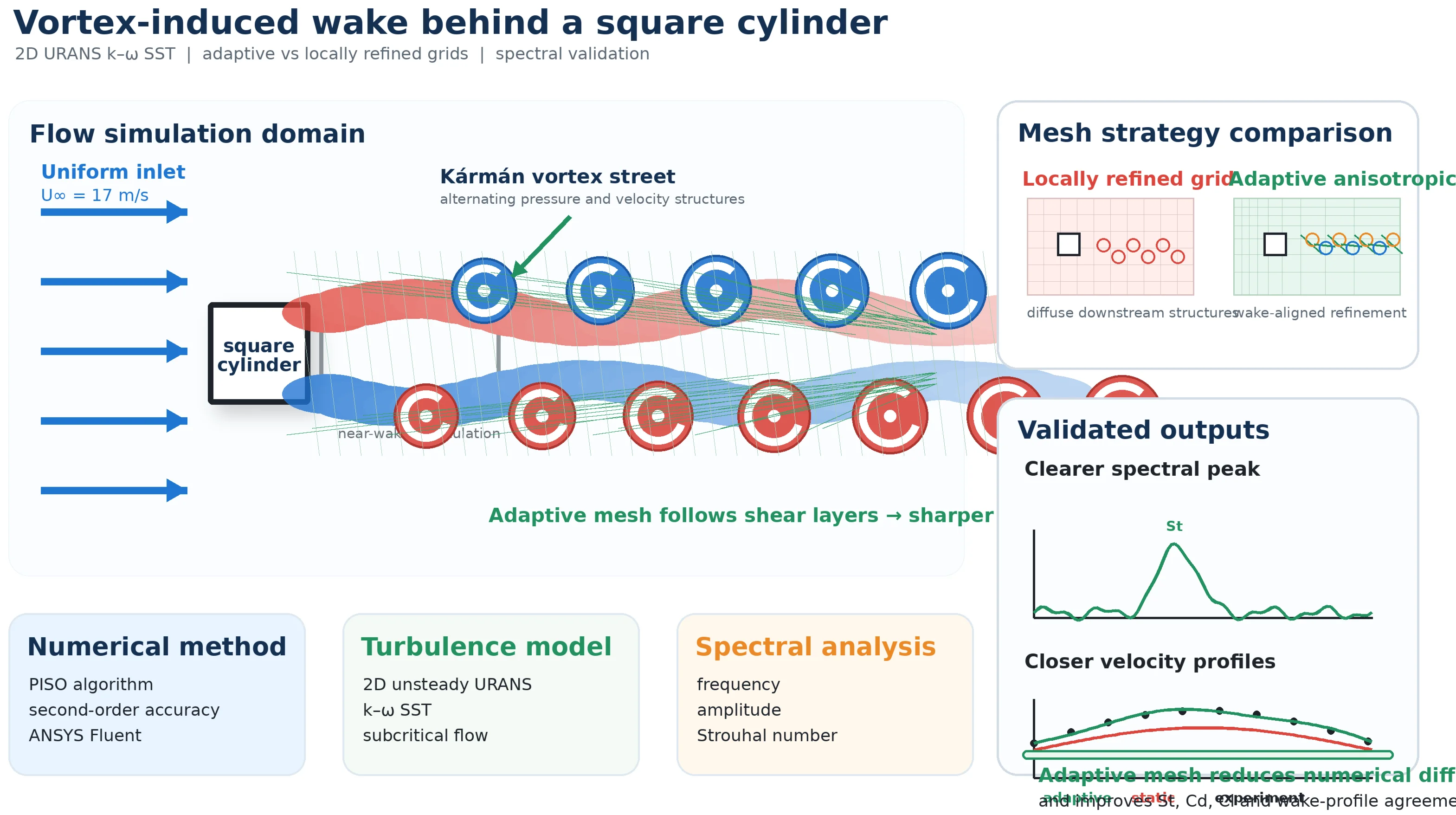
Adaptive anisotropic meshing improves wake resolution behind a square cylinder.
The 2D URANS k–ω SST model captures Kármán vortex shedding and spectral behavior.
Adaptive grids reduce numerical diffusion and better match experimental velocity profiles.
Strouhal number, drag, and lift predictions are improved using Hessian-based adaptation.

1. Introduction

Thin-walled structures (e.g., buildings, chimneys, cables) often interact aerodynamically in groups and have significant effects on pressures and forces. Even simple body configurations exhibit the basic characteristics of turbulent flow, such as flow separation, vortex shedding, and instability [1-2]. Flow past a circular cylinder is a classic case for studying vortex streets, while a square cylinder differs due to fixed separation at sharp edges. A square cylinder at $R e \approx$ 2.2×10⁴ is a common benchmark [5-6]. For two side-by-side cylinders, flow depends on both 𝑅𝑒 and spacing $(T / d)$ , leading to regimes like single-body behavior, gap flow (“flip-flop”), and paired vortex shedding, each affecting forces and frequencies [7-9]. Experiments provide reliable data but are limited, while numerical methods allow broader studies. DNS is accurate but very expensive, LES reduces cost but remains demanding [10-16], and RANS is widely used for practical cases [17-19]. The $k$ - $ω$ SST model combines near-wall and free-flow advantages and handles separation well, though results depend on mesh and setup [20-22]. Other models like RSM may improve wake predictions but still have limitations [23-24]. Mesh quality is critical: resolving wakes requires proper $y^{+}$ , time step, and grid distribution. Two main approaches are local refinement and adaptive anisotropic meshing, which better captures gradients and improves spectral accuracy at similar cost.

This paper studies flow past a square cylinder using unsteady 2D URANS $k$ - $ω$ SST, comparing these two mesh strategies. Validation uses St, Cd, Cl and velocity profiles. Both capture the Karman vortex street, but the adaptive mesh better resolves the near wake and spectra. Limitations of 2D URANS for inherently 3D flows are also discussed.

2. Physical and mathematical formulation of the problem

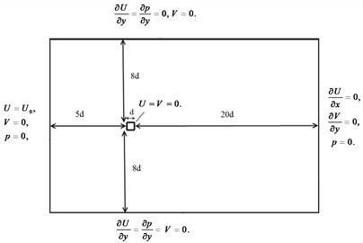
We consider the flow around a single square cylinder with side 𝑑 (in calculations: $d =$ 0.042 m) by a two-dimensional flow at an inlet velocity of $U_{\infty} =$ 17 m/s (subcritical regime, $R e \approx$ 4.7×10⁴). The computational domain is defined in a Cartesian coordinate system (𝑥, 𝑦) so as to exclude the influence of distant boundaries on the wake and forces: inlet: $x = - 5 d$ , outlet: $x = + 20 d$ , top/bottom: $y = \pm 8 d$ . This choice ensures low blockage: $β = d / H \approx$ 1/16 ≈ 6.25 % at a section height of $H = 16 d$ , which is acceptable for reproducing free flow. The center of the cylinder is located at (𝑥, 𝑦) = (0, 0); its ribs are oriented parallel to the axes (angle of attack $α =$ 0) [7].

Fig. 1Two-dimensional computational domain and boundary conditions

2.1. Boundary conditions

Velocity-inlet. A uniform velocity profile of $U_{\infty} =$ 17 m/s and low turbulence corresponding to a wind tunnel are specified: intensity $T I =$ 0.5 % and integral length $L \approx$ $0.07 d$ . In the $k$ - $ω$ parameterization: $k = 1.5 (U_{\infty} T I)^{2}$ , $ω = k / (C_{μ} / 4 L)$ , $C_{μ} =$ 0.09. Pressure-outlet. Zero excess static pressure (0 Pa). The backflow parameters are consistent with the inlet: $T I =$ 0.5 %, $L \approx 0.07 d$ . Top/bottom. Symmetry-type boundaries (sliding plane) to eliminate parasitic viscous effects from the “pipe walls”. Cylinder surface. No-slip, isothermal solid wall.

2.2. Mathematical model

A RANS-based approach is used, where flow variables are decomposed into mean and fluctuating parts to account for turbulence without resolving all scales. Averaging yields equations for mean velocity and pressure, including Reynolds stresses that represent turbulence effects. To close the system, the $k$ - $ω$ SST model [20-22] is applied, enabling reasonable prediction of separation, turbulence anisotropy, and streamline curvature effects.

The equation of conservation of mass and momentum, which describes the change in the velocity of a fluid under the influence of external and internal forces:

1

\{\begin{array}{l} \frac{\partial {\bar{u}}_{i}}{\partial x_{i}} = 0, \\ \frac{\partial {\bar{u}}_{i}}{\partial t} + {\bar{u}}_{j} \frac{\partial {\bar{u}}_{i}}{\partial x_{j}} = - \frac{1}{ρ} \frac{\partial \bar{p}}{\partial x_{i}} + ν \frac{\partial^{2} {\bar{u}}_{i}}{\partial x_{j} \partial x_{i}} + \frac{1}{ρ} \frac{\partial}{\partial x_{i}} (2 μ_{t} (S_{i j} - (\frac{\partial u_{k}}{3 \partial x_{k}}) δ_{i j}) - \frac{2}{3} ρ k δ_{i j}), \end{array}

where ${\bar{u}}_{i}$ – components of the average velocity field, $\bar{p}$ – average pressure, $ν$ – kinematic viscosity, $ρ$ – density.

2.3. Turbulence models

The SST turbulence model by Menter [20] combines the advantages of the $k$ - $ε$ and $k$ - $ω$ models using a hybrid approach: $k$ - $ω$ is applied near walls for boundary layer accuracy, while $k$ - $ε$ is used in the free-flow region for stability:

2

\{\begin{array}{l} \frac{\partial (ρ k)}{\partial t} + \frac{\partial (ρ u_{j} k)}{\partial x_{j}} = P - β^{*} ρ ω k + \frac{\partial}{\partial x_{j}} [(μ + σ_{k} μ_{t}) \frac{\partial k}{\partial x_{j}}], \\ \frac{\partial (ρ ω)}{\partial t} + \frac{\partial (ρ u_{j} ω)}{\partial x_{j}} = \frac{γ}{ν_{t}} P - β ρ ω^{2} + \frac{\partial}{\partial x_{j}} [(μ + σ_{ω} μ_{t}) \frac{\partial ω}{\partial x_{j}}] + 2 (1 - F_{1}) \frac{ρ σ_{ω 2}}{ω} \frac{\partial k}{\partial x_{j}} \frac{\partial ω}{\partial x_{j}} . \end{array}

The remaining coefficients and functions were presented in the article [20].

2.4. Computational grids

The paper compares two partitioning strategies: (A) a statically locally dense mesh near a cylinder (Fig. 2) and (B) an adaptive anisotropic mesh (Hessian-based) with preservation of wall layers [25-26].

Fig. 2Statically locally compacted mesh near the cylinder

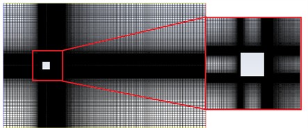
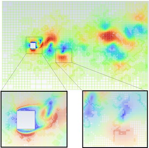
Mesh A - locally refined near the cylinder. Uses a triangular/polygonal mesh with prismatic inflation layers (15-20 layers, growth 1.20-1.25, $y^{+} \approx 1$ ). Edge step $Δ s ≲ 0.01 d$ . The wake (0-10𝑑) has moderate refinement, coarsening smoothly downstream. Quality: skewness <0.4, angle >30°, orthogonality >0.2. Total cells $\approx$ 2.5×10⁴. Mesh B – adaptive anisotropic (Hessian-based). Starts similar to Mesh A (same layers, $y^{+} \approx 1$ ), then adapts in Fluent using a combined Hessian indicator (velocity/pressure). Boundary layers are preserved. Sizes: $Δ_{m i n} \approx$ (0.006-0.01) $d$ , $Δ_{m a x} \approx 0.2 d$ . Adaptation every 50–100 steps, refining ~20-30 % and coarsening ~10-15 % of cells. After 3-5 cycles, a wake-aligned mesh forms with controlled cell growth.

Fig. 3Adaptive (anisotropic, Hessian)

3. Solution method

Finite volume solution (ANSYS Fluent): Pressure–velocity coupling: PISO. Time: Second-Order Implicit (unsteady URANS). Gradients: Least Squares Cell-Based. Pressure: Second-Order. Convection (momentum, 𝑘, 𝜔): Second-Order Upwind. (Note: For URANS/SST, second-order convection minimizes numerical diffusion and correctly reproduces the stall frequency.) Rhie-Chow interpolation by default; skewness/neighbour correction = 1 (for high grid skew, 2) [27-32].

4. Results and discussion

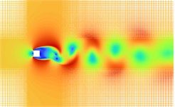
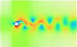
Fig. 4 instantaneous flow fields around a square cylinder for several phases of one stall period $t / T =$ {0.10; 0.15; 0.20 s} with the superposition of the computational grid.

Fig. 4Instantaneous flow fields around a square cylinder at several phases of one stall period

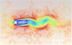
a) 0.1 s

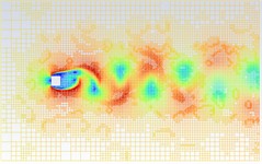
b) 0.15 s

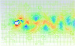
c) 0.2 s

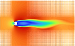
d) 0.1 s

e) 0.15 s

f) 0.2 s

The top rows show an adaptive (anisotropic, Hessian-based) grid, while the bottom rows use static local refinement near the cylinder. Flow structures (velocity/vorticity and pressure) illustrate vortex formation and shedding, the recirculation zone, and alternating pressure regions of the Karman street. With adaptation, the grid refines in shear layers and the wake while coarsening elsewhere, giving sharper resolution of fine structures and stable vortex amplitude and spacing. In contrast, the static grid concentrates resolution near the body; downstream, shear layers thicken and structures become more diffuse. The pressure field shows high pressure at the stagnation point, suction at sharp edges, and alternating low/high-pressure regions in the wake aligned with vortex shedding.

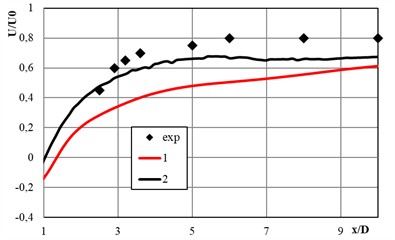
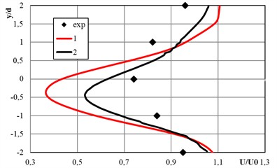
Fig. 5 shows a comparison of the calculated longitudinal velocity profiles $U_{x} / U_{0}$ with the experiment. (a) Reconstruction of $⟨U_{x}⟩ t / U_{0}$ along the wake axis behind a square cylinder (time averaging along the line $y =$ 0, coordinate 𝑥/𝐷). (b) Transverse profile $U_{x} / U_{0}$ on the section $x / D =$ 4 in the coordinate $y / d$ .

Marker exp – experimental data; curve 1 – statically locally densed grid (red), curve 2 – adaptive anisotropic grid (black). Normalization: $U_{0}$ – inlet velocity, $D = d$ – cylinder edge size. It is evident that the adaptive grid better reproduces the growth of $⟨U_{x}⟩ t$ along the wake axis and the steepness of gradients in shear layers; with static densed grid, an underestimation of $U_{x} / U_{0}$ in the near wake and a smoother transverse profile are observed.

Fig. 6 shows the transverse profiles of the transverse velocity component $U_{y} / U_{0}$ : (a) section $x / D =$ 1; (b) section $x / D =$ 2. Marker exp – experiment; curve 1 – statically locally densed grid; curve 2 – adaptive.

The profiles exhibit a classic S-shaped antisymmetry about the $y =$ 0 axis: positive values at the top and negative values at the bottom due to alternating vortex shedding. At $x / D =$ 1, $|U_{y}|$ extrema form in shear layers at $y / D \approx$ ±(1-1.5); the adaptive grid more accurately reproduces their amplitude and position, while static compaction underestimates $|U_{y}|$ and smooths the profile. At $x / D =$ 2, a wake broadening and a weakening amplitude are observed, while the adaptive grid preserves steeper gradients and better agreement with experiment.

Fig. 5Comparison of the calculated longitudinal velocity profiles Ux/U0 with the experiment

a)

b)

Fig. 6Transverse profiles of the transverse velocity component Uy/U0

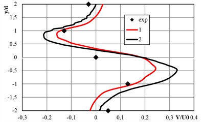
a) Section 𝑥/𝐷 = 1

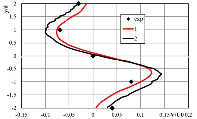
b) Section 𝑥/𝐷 = 2

5. Conclusions

The study shows that the unsteady 2D URANS $k$ - $ω$ SST model reliably reproduces the Karman vortex street behind a square cylinder, with both static and adaptive grids giving consistent velocity and pressure fields. The adaptive (Hessian-based) grid improves accuracy by aligning with the flow, reducing numerical diffusion, and better capturing the near wake and spectral features: the Strouhal number matches experiments more closely, peaks are more stable, and signals are clearer. Drag Cd, lift Cl, and velocity profiles $(U_{x} / U_{0}, U_{y} / U_{0})$ also agree better with experiments, while static grids give smoother results. Accurate results require $y^{+} \approx$ 1, PISO coupling, second-order schemes, and $Δ t$ with CFL ≤ 1 (~200 steps per period). Adaptive meshing has similar cost to static refinement but higher accuracy. A key limitation is the 2D URANS approach, which cannot capture full 3D effects and flow intermittency.

References

K. Shimada and T. Ishihara, “Application of a modified k-e model to the prediction of aerodynamic characteristics of rectangular cross-section cylinders,” Journal of Fluids and Structures, Vol. 16, No. 4, pp. 465–485, 2002, https://doi.org/10.1006/jfls.2001.0433

Publisher
H. C. Lim, T. G. Thomas, and I. P. Castro, “Flow around a cube in a turbulent boundary layer: LES and experiment,” Journal of Wind Engineering and Industrial Aerodynamics, Vol. 97, No. 2, pp. 96–109, 2009, https://doi.org/10.1016/j.jweia.2009.01.001

Publisher
S. Huang and Q. S. Li, “A new dynamic one-equation subgrid-scale model for large eddy simulations,” International Journal for Numerical Methods in Engineering, Vol. 81, No. 7, pp. 835–865, 2010, https://doi.org/10.1002/nme.2715

Publisher
K. Nozawa and T. Tamura, “Large eddy simulation of the flow around a low-rise building immersed in a rough-wall turbulent boundary layer,” Journal of Wind Engineering and Industrial Aerodynamics, Vol. 90, No. 10, pp. 1151–1162, 2002, https://doi.org/10.1016/s0167-6105(02)00228-3

Publisher
S. Liao, L. Wang, G. Yang, and W. Lin, “A third-order characteristic-based-split finite element scheme of Spalart-Allmaras model and its application to flow past crescent iced 4-bundled conductors,” Advances in Aerodynamics, Vol. 8, No. 1, p. 4, 2026, https://doi.org/10.1186/s42774-025-00215-6

Publisher
A. Sohankar, L. Davidson, and C. Norberg, “Large eddy simulation of flow past a square cylinder: comparison of different subgrid scale models,” Journal of Fluids Engineering, Vol. 122, No. 1, pp. 39–47, 2000, https://doi.org/10.1115/1.483224

Publisher
M. M. Alam, Y. Zhou, and X. W. Wang, “The wake of two side-by-side square cylinders,” Journal of Fluid Mechanics, Vol. 669, pp. 432–471, 2011, https://doi.org/10.1017/s0022112010005288

Publisher
O. Inoue, M. Mori, and N. Hatakeyama, “Aeolian tones radiated from flow past two square cylinders in tandem,” Physics of Fluids, Vol. 18, No. 4, p. 046104, 2006, https://doi.org/10.1063/1.2187446

Publisher
S. C. Yen and J. H. Liu, “Wake flow behind two side-by-side square cylinders,” International Journal of Heat and Fluid Flow, Vol. 32, No. 1, pp. 41–51, 2011, https://doi.org/10.1016/j.ijheatfluidflow.2010.09.005

Publisher
I. Afgan, Y. Kahil, S. Benhamadouche, and P. Sagaut, “Large eddy simulation of the flow around single and two side-by-side cylinders at subcritical Reynolds numbers,” Physics of Fluids, Vol. 23, No. 7, p. 075101, 2011, https://doi.org/10.1063/1.3596267

Publisher
L. Zou, Y.-F. Lin, and K. Lam, “Large-eddy simulation of flow around cylinder arrays at a subcritical Reynolds number,” Journal of Hydrodynamics, Vol. 20, No. 4, pp. 403–413, 2008, https://doi.org/10.1016/s1001-6058(08)60074-8

Publisher
A. Li and G. Ahmadi, “Dispersion and deposition of spherical particles from point sources in a turbulent channel flow,” Aerosol Science and Technology, Vol. 16, No. 4, pp. 209–226, Jan. 1992, https://doi.org/10.1080/02786829208959550

Publisher
L. Tian and G. Ahmadi, “Particle deposition in turbulent duct flows-comparisons of different model predictions,” Journal of Aerosol Science, Vol. 38, No. 4, pp. 377–397, Apr. 2007, https://doi.org/10.1016/j.jaerosci.2006.12.003

Publisher
H. Zhang, G. Ahmadi, F.-G. Fan, and J. B. Mclaughlin, “Ellipsoidal particles transport and deposition in turbulent channel flows,” International Journal of Multiphase Flow, Vol. 27, No. 6, pp. 971–1009, Jun. 2001, https://doi.org/10.1016/s0301-9322(00)00064-1

Publisher
G. Tryggvason, R. Scardovelli, and S. Zaleski, Direct Numerical Simulations of Gas-Liquid Multiphase Flows. Cambridge University Press, 2001, https://doi.org/10.1017/cbo9780511975264

Publisher
L. Hájek, J. Karel, M. Klíma, and D. Trdlička, “Comparison of new RANS-LES hybrid methods on a tandem cylinder problem using rough meshes,” Applied and Computational Mechanics, Vol. 18, No. 2, Jan. 2024, https://doi.org/10.24132/acm.2024.893

Publisher
J. Richmond-Bryant, “Verification testing in computational fluid dynamics: an example using Reynolds-averaged Navier-Stokes methods for two-dimensional flow in the near wake of a circular cylinder,” International Journal for Numerical Methods in Fluids, Vol. 43, No. 12, pp. 1371–1389, 2003, https://doi.org/10.1002/fld.568

Publisher
P. Spalart and S. Allmaras, “A one-equation turbulence model for aerodynamic flows,” in 30th Aerospace Sciences Meeting and Exhibit, Vol. 92, p. 0349, 1992, https://doi.org/10.2514/6.1992-439

Publisher
Z. Han, D. Zhou, J. Tu, C. Fang, and T. He, “Flow over two side-by-side square cylinders by CBS finite element scheme of Spalart-Allmaras model,” Ocean Engineering, Vol. 87, pp. 40–49, Sep. 2014, https://doi.org/10.1016/j.oceaneng.2014.05.006

Publisher
F. R. Menter, “Two-equation eddy-viscosity turbulence models for engineering applications,” AIAA Journal, Vol. 32, No. 8, pp. 1598–1605, Aug. 1994, https://doi.org/10.2514/3.12149

Publisher
P. E. Smirnov and F. R. Menter, “Sensitization of the SST turbulence model to rotation and curvature by applying the spalart-shur correction term,” Journal of Turbomachinery, Vol. 131, No. 4, p. 041010, Oct. 2009, https://doi.org/10.1115/1.3070573

Publisher
A. Fellague Chebra, M. Braikia, A. Khelil, M. Bedrouni, and D. Zied, “Numerical study of turbulent flows around a cubic obstacle blown from a variable geometry jets diffuser,” Applied and Computational Mechanics, Vol. 18, No. 1, Jan. 2024, https://doi.org/10.24132/acm.2024.837

Publisher
M. N. Haque, “Applicability of unsteady RANS for predicting flow fields around cylinders,” in Proceedings of the 4th International Conference on Civil Engineering for Sustainable Development (ICCESD 2018), 2018.

Search CrossRef
A. Rusdin, “Computation of turbulent flow around a square block with standard and modified k-ε turbulence models,” International Journal of Automotive and Mechanical Engineering, Vol. 14, No. 1, pp. 3938–3953, 2022, https://doi.org/10.15282/ijame.14.1.2017.10.0320

Publisher
P. J. Frey and F. Alauzet, “Anisotropic mesh adaptation for CFD computations,” Computer Methods in Applied Mechanics and Engineering, Vol. 194, No. 48-49, pp. 5068–5082, Nov. 2005, https://doi.org/10.1016/j.cma.2004.11.025

Publisher
L. Formaggia, S. Micheletti, and S. Perotto, “Anisotropic mesh adaptation in computational fluid dynamics: Application to the advection-diffusion-reaction and the Stokes problems,” Applied Numerical Mathematics, Vol. 51, No. 4, pp. 511–533, Dec. 2004, https://doi.org/10.1016/j.apnum.2004.06.007

Publisher
Z. M. Malikov, M. E. Madaliev, D. P. Navruzov, and K. Adilov, “Numerical study of an axisymmetric jet based on a new two-fluid turbulence model,” in AIP Conference Proceedings, Vol. 2637, No. 1, p. 040023, Jan. 2022, https://doi.org/10.1063/5.0118473

Publisher
Z. M. Malikov, M. E. Madaliev, S. L. Chernyshev, and A. A. Ionov, “Validation of a two-fluid turbulence model in Comsol multiphysics for the problem of flow around aerodynamic profiles,” Scientific Reports, Vol. 14, No. 1, p. 2306, Jan. 2024, https://doi.org/10.1038/s41598-024-52673-5

Publisher
M. Madaliev, Z. Abdulkhaev, K. Kurpayanidi, A. Abdullayev, and A. Ilyosov, “Study of the SST turbulence model for the 2D NASA wall-mounted hump separated FLOW problem with plenum case,” E3S Web of Conferences, Vol. 508, p. 06007, Apr. 2024, https://doi.org/10.1051/e3sconf/202450806007

Publisher
E. Madaliev, M. Madaliev, A. Akramov, S. Umurqulov, and S. Qurbonova, “Numerical simulation of the flow in a flat suddenly expanding channel based on a two-fluid turbulence model,” E3S Web of Conferences, Vol. 508, No. 1, p. 06001, Mar. 2024, https://doi.org/10.1051/e3sconf/202450806001

Publisher
M. Madaliev, “Simulation of flow around a square cylinder using the DES method with an adaptive mesh,” Journal of Construction and Engineering Technology, Vol. 4, No. 1, pp. 1–6, 2026, https://doi.org/10.24412/2181-4473-2026.4.101

Publisher
E. Madaliev, M. Madaliev, S. Raxmankulov, and S. Raxmonkulova, “Turbulent mixing of two plane flows based on the SST turbulence model,” E3S Web of Conferences, Vol. 452, p. 02012, Nov. 2023, https://doi.org/10.1051/e3sconf/202345202012

Publisher

About this article

Received

March 31, 2026

Accepted

April 15, 2026

Published

July 16, 2026

SUBJECTS

Mathematical models in engineering

DOI

https://doi.org/10.21595/vp.2026.26474

Keywords

Navier-Stokes equations

SST

RANS

ANSYS

Acknowledgements

The authors have not disclosed any funding.

Data Availability

The datasets generated during and/or analyzed during the current study are available from the corresponding author on reasonable request.

Conflict of interest

The authors declare that they have no conflict of interest.

This is an open access article distributed under the Creative Commons Attribution License, which permits unrestricted use, distribution, and reproduction in any medium, provided the original work is properly cited.

Previous article in issue Previous Next article in issue Next

M. Madaliev, E. Mamurov, R. Tadjibayev, A. Gaynazarov, A. Mamirov, and G. Nishonova, “Numerical analysis of vortex-induced flow structures and their spectral characteristics behind a square cylinder using adaptive and locally refined grids,” Vibroengineering Procedia, Vol. 63, pp. 179–185, Jul. 2026, https://doi.org/10.21595/vp.2026.26474

Copy Extrica

Copied to clipboard!

TY  - JOUR
DO  - 10.21595/vp.2026.26474
UR  - https://doi.org/10.21595/vp.2026.26474
TI  - Numerical analysis of vortex-induced flow structures and their spectral characteristics behind a square cylinder using adaptive and locally refined grids
T2  - Vibroengineering Procedia
AU  - Madaliev, Murodil
AU  - Mamurov, Eldor
AU  - Tadjibayev, Rasul
AU  - Gaynazarov, Abdulvasiy
AU  - Mamirov, Abdurashid
AU  - Nishonova, Gazaloy
PY  - 2026
DA  - 2026/07/16
PB  - Extrica
SP  - 179-185
VL  - 63
SN  - 2345-0533
SN  - 2538-8479
ER  - 

Copy Ris

Copied to clipboard!

@article{doi_10.21595/vp.2026.26474,
  title = {Numerical analysis of vortex-induced flow structures and their spectral characteristics behind a square cylinder using adaptive and locally refined grids},
  author = {Madaliev, Murodil and Mamurov, Eldor and Tadjibayev, Rasul and Gaynazarov, Abdulvasiy and Mamirov, Abdurashid and Nishonova, Gazaloy},
  journal = {Vibroengineering Procedia},
  year = {2026},
  month = {7},
  volume = {63},
  pages = {179--185},
  doi = {10.21595/vp.2026.26474},
  url = {https://doi.org/10.21595/vp.2026.26474},
  publisher = {Extrica},
  issn = {2345-0533},
  eissn = {2538-8479},
}

Copy Bibtex

Copied to clipboard!

[1]M. Madaliev, E. Mamurov, R. Tadjibayev, A. Gaynazarov, A. Mamirov, and G. Nishonova, “Numerical analysis of vortex-induced flow structures and their spectral characteristics behind a square cylinder using adaptive and locally refined grids,” Vibroengineering Procedia, vol. 63, pp. 179–185, Jul. 2026, doi: 10.21595/vp.2026.26474.

Copy IEEE

Copied to clipboard!

Madaliev, Murodil, Eldor Mamurov, Rasul Tadjibayev, Abdulvasiy Gaynazarov, Abdurashid Mamirov, and Gazaloy Nishonova. “Numerical analysis of vortex-induced flow structures and their spectral characteristics behind a square cylinder using adaptive and locally refined grids.” Vibroengineering Procedia 63 (2026): 179–185. https://doi.org/10.21595/vp.2026.26474.

Copy Chicago

Copied to clipboard!

Numerical analysis of vortex-induced flow structures and their spectral characteristics behind a square cylinder using adaptive and locally refined grids

Abstract

Highlights

1. Introduction

2. Physical and mathematical formulation of the problem

2.1. Boundary conditions

2.2. Mathematical model

2.3. Turbulence models

2.4. Computational grids

3. Solution method

4. Results and discussion

5. Conclusions

References

About this article

Related Articles