Intelligent risk-oriented predictive diagnostics system based on vibration signal analysis

2.1. Stochastic model of the vibration process

We consider a dynamic mechanical system whose state is determined by a parametric vector $\theta$. The measured vibration signal is represented as:

where $s(t;\theta )$ is a deterministic component reflecting the dynamic response of a structure or equipment unit, $\theta$ is a state parameter (wear, raceway crack), and $\epsilon \left(t\right)$ is an additive random component modeled by a stationary Gaussian process with zero mean and variance ${\sigma }^2$ [19].

The presence of a defect leads to a change in the parameters of the dynamic system:

In the presence of a defect, the frequencies of characteristic impacts change [1, 2]: BPFO – outer ring defect, BPFI – inner ring defect, BSF – rolling element defect. To increase the information content, the signal is transformed into a time-frequency space [20]:

where $\mathrm{\Phi }(\cdot )$ is the STFT operator or wavelet transform. The resulting feature space ${\rm Z}\subset {\mathbb{R}}^d$ is used to construct a probabilistic classifier.

2.2. Bayesian formalization of decision making

Let the model generate the posterior probability of a defect:

The decision rule is defined by the threshold $t$:

Taking into account asymmetric losses, the Bayesian risk functional is introduced [9, 21]:

where $C_{FN}$ is the cost of missing a bearing defect, $C_{FP}$ is the cost of a false alarm, and ${\pi }_i$ are the prior probabilities of the classes.

For a posterior-calibrated score, the optimal threshold follows directly from the comparison of conditional risks. Deciding $H_1$ for an observation $z$ incurs the expected cost $C_{FP}\left(1-p\left(z\right)\right)$, whereas deciding $H_0$ incurs $C_{FN}p\left(z\right)$; choosing $H_1$ whenever $C_{FN}p\left(z\right)\ge C_{FP}\left(1-p\left(z\right)\right)$ yields:

Eq. (7) contains no prior probabilities: for a score calibrated as the posterior Eq. (4), the priors are already embedded in $p\left(z\right)$ through the Bayes rule, and re-introducing ${\pi }_0$ and ${\pi }_1$ into the threshold would double-count the class prevalence. The prior-dependent form of the decision rule is the likelihood-ratio test discussed in Section 2.4, where the threshold $\eta =\frac{C_{FP}{\pi }_0}{C_{FN}{\pi }_1}$ is applied to the likelihood ratio rather than to the posterior probability.

Thus, the problem of choosing the threshold $t$ is reduced to minimizing the risk functional [15].

2.3. Variational derivation of the optimality condition

Consider the variation of the threshold $t\to t+\delta t$. The first risk variation is defined as follows:

The extremum condition is defined as follows:

Taking into account the dependence of $TPR\left(t\right)$ and $FPR\left(t\right)$ on the threshold, we obtain:

This ratio determines the optimal operating point on the ROC curve [22, 23]. This means that the operating point on the ROC curve is determined by the economic ratio of the cost of errors.

2.4. Relationship with the Neyman-Pearson criterion

The classic Neyman-Pearson criterion is formulated as a problem of optimally distinguishing between two hypotheses:

– $H_0:$normal bearing condition (no defect).

– $H_1:$presence of a defect (damage to the raceway or rolling elements).

The optimal decision rule is based on the likelihood ratio $\mathrm{\Lambda }\left(x\right)=\frac{f(x\mid H_1)}{f(x\mid H_0)}\gtrless \eta$, where $f\left(x\right|H_i$ is the density function of the observed signal under the corresponding hypotheses, and 𝜂 is the threshold, defined as $\eta =\frac{C_{FP}{\pi }_0}{C_{FN}{\pi }_1}$.

According to the Neyman-Pearson theorem, this rule is optimal in the sense of maximizing the probability of detecting a defect TPR and for a fixed false alarm rate FPR. Thus, risk-based optimization is a generalization of the Neyman-Pearson theorem for probabilistic classifiers.

2.5. Geometric interpretation

In ROC space, the Neyman-Pearson criterion corresponds to choosing a point on the ROC curve for a fixed FPR. The set of points with a constant value of the risk functional Eq. (6), $R\left(t\right)=R=$ const, forms a family of isorisk lines in ROC space:

where $a=1-\frac{R}{C_{FN}{\pi }_1}$ and $b=\frac{C_{FP}{\pi }_0}{C_{FN}{\pi }_1}>$ 0. Isorisk lines therefore have a positive slope equal to the cost ratio in Eq. (10), and the risk $R$ decreases as the intercept $a$ increases, i.e., as the line is translated toward the upper-left corner of ROC space.

The optimal operating point is the point at which the isorisk line with the largest intercept $a$ still touches the ROC curve; at this tangency point the slope of the ROC curve equals $b$, which reproduces the optimality condition Eq. (10). Thus, the Neyman-Pearson criterion fixes the FPR, and the risk-based approach minimizes the expected damage. A key feature of the problem is the strong asymmetry of losses:

since missing a defect can lead to equipment failure, emergency shutdown, and significant economic losses. As a result, the optimal threshold shifts toward earlier defect detection (increasing system sensitivity).

3.1. Conceptual structure

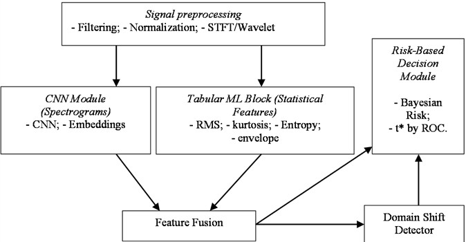
The proposed architecture of the hybrid diagnostic system includes the following modules:

– Signal preprocessing module.

– Neural network unit for extracting time-frequency features.

– Table module for statistical characteristics.

– Representation fusion mechanism.

– Risk-based decision-making unit.

This modular structure ensures the interpretability and robustness of the model [11, 12].

3.2. CNN Block

A convolutional neural network (CNN) is used to automatically extract informative features from vibration signals represented in the time-frequency domain. The input data is a spectrogram obtained using the short-time Fourier transform (STFT) [7]:

This CNN representation allows for the mapping and extraction of local variations in the signal’s time-frequency characteristics that occur during the development of bearing defects, which correspond to bearing wear, misalignment, cracks, and dynamic imbalance. Bearing defects manifest themselves as impulse effects, modulated harmonic components, and broadband energy spikes. These effects result in characteristic patterns in the spectrogram: vertical stripes (shock pulses), horizontal lines (harmonics), and local energy concentrations. CNN effectively identifies such structures through local convolution operations. The typical block architecture includes a sequence of layers: convolutional layers – $h_1=\sigma (W_1*S+b_1)$, pooling layers – $h_2=Pool\left(h_1\right)$, and deep convolutional representations – $h_I=\sigma (W_I*h_{I-1}+b_I)$, where * is the convolution operation, $W_I$ are the convolution kernels, $b_I$ are the biases, and $\sigma$ is the nonlinear activation function (ReLU).

After passing through the convolutional layers, a feature vector $z_{CNN} = {\phi }_{CNN}\left(S\right(f, t\left)\right)$ is formed. This vector contains local time-frequency correlations, features of impact processes, and spectral modulation information. Given representative labeled training data, the CNN learns discriminative time-frequency patterns that are statistically associated with the characteristic defect frequency bands (BPFO, BPFI, BSF), their harmonics and amplitude modulations; the network does not identify these frequencies analytically, and attributing the learned filters to specific physical mechanisms requires separate validation. Unlike classical methods such as spectral analysis or envelope detection, CNNs do not require manual feature selection, which increases the model’s versatility. To improve generalization, regularization methods such as Dropout ($z\text{'}= z\odot m$) and Batch Normalization ($\widehat{h}=(h-\mu )/\sigma$) are used. These methods reduce overfitting, increase robustness to noise, and improve the model's transferability across different operating conditions. The CNN output is used as part of a hybrid architecture: $z=[z_{CNN},{ z}_{stat}]$, where ${ z}_{stat}$ are statistical features (RMS, kurtosis, etc.). This combined vector is fed to a fusion head – a two-layer fully connected network (128 → 64 → 1 neurons, ReLU activations, sigmoid output) – which generates the posterior probability (4); the output probabilities are additionally calibrated on the validation set by Platt scaling [24, 25].

The CNN block is implemented on industrial computing hardware (IPC) and provides a processing time of $T_{CNN}\approx$ 10-15 ms for a single signal window. This enables the model to be used in near-real-time mode. The CNN block automatically extracts features from spectrograms, takes into account the physical properties of vibration processes, improves the accuracy of bearing diagnostics, and ensures robustness to noise and signal variability. This makes it a key element of an intelligent predictive diagnostics system.

3.3. Statistical feature tabular block

Classical diagnostic indicators are used to complement the CNN embedding [26]. The tabular block is implemented as a gradient-boosting decision-tree ensemble (XGBoost; 200 trees, maximum depth 4, learning rate 0.1, subsampling rate 0.8) operating on a 12-dimensional vector of statistical features computed for each window: RMS, variance, skewness, kurtosis, crest factor, impulse factor, shape factor, clearance factor, peak-to-peak amplitude, spectral entropy, the envelope-spectrum energy in the BPFO/BPFI/BSF bands, and the amplitude of the dominant spectral component. Combining neural-network and statistical features improves the robustness of the system [27].

Fig. 1 shows a system that includes a vibration signal pre-processing module, two parallel feature extraction channels (CNN for spectrograms and tabular ML for statistical indicators), a representation fusion layer, a domain (distribution) shift detector, and a risk-based decision-making unit. This unit calculates an adaptive classification threshold $t^{*}$ based on the Bayesian risk minimization condition, taking into account asymmetric error costs and operational constraints [13].

Fig. 1Hybrid diagnostic system architecture

3.4. Domain shift detection mechanism

Under real-world bearing operating conditions, the distribution of vibration signals can vary due to variations in load, rotational speed, mounting conditions, and sensor characteristics [28]. This leads to the phenomenon of distributional (domain) shift, in which $P_{train}\ne P_{test}$ holds. The Kullback-Leibler divergence is used to quantify the degree of difference between the distributions:

In the continuous case, the expression is written in integral form:

A domain shift is detected when the following condition is met:

where $\tau$ is a detection threshold determined on the validation set. In the proposed system, the divergence is not estimated in the raw high-dimensional feature space, where KL estimates are known to be unstable; instead, Eq. (14) is applied to the one-dimensional distribution of the calibrated score $p\left(z\right)$ and, as a control, to each standardized statistical feature separately. The distributions are estimated over a sliding window of the last $N=$ 2000 processed signal windows using histograms with $B=$ 32 equal-width bins and Laplace smoothing, which guarantees a finite estimate; the threshold $\tau$ is set to the 99th percentile of the bootstrap distribution of the divergence computed between disjoint subsamples of the validation data.

When this threshold is exceeded, the model adaptation mechanism is activated. Instead of completely retraining the model, a more computationally efficient approach is proposed: decision-threshold adaptation. For a posterior-calibrated score, the risk-optimal threshold is given by Eq. (7) and contains no prior probabilities. A domain shift, however, changes the class priors ${\pi }_0\to {\pi }_0^{\text{'}}$, ${\pi }_1\to {\pi }_1^{\text{'}}$ relative to the priors under which the score $p\left(z\right)$ was calibrated. Re-deriving the decision rule for the training-calibrated score under the new priors – re-weighting the posterior by the prior ratios and applying Eq. (7) – yields the adapted threshold:

Eq. (17) reduces to Eq. (7) when the priors do not change (${\pi }_0^{\text{'}}={\pi }_0$, ${\pi }_1^{\text{'}}={\pi }_1$): the class prevalence enters only through the ratio of the deployment priors to the training priors and is therefore counted exactly once. In addition to the priors, the operating characteristics themselves change under shift, TPR → TPR′, FPR → FPR′; the effect of such perturbations on the risk is bounded in Proposition 1 below.

Under industrial operation conditions, cost parameters are dynamic and depend on the current state of the equipment. In particular, the cost of missing a defect increases with increasing load and the cost of a false alarm decreases with scheduled maintenance. This can be formalized as follows:

where $L$ is the load level, $S$ is the state of the production process.

Then the adaptive threshold can be written as a function:

The detection and adaptation mechanism is implemented in the following sequence:

– Estimate the current distribution of the input data $P_{test}\left(x\right)$.

– Calculate the divergence $D_{KL}(P_{train}\parallel P_{test})$.

– Check the condition $D_{KL}>\tau$.

– When a shift is detected, the prior probabilities ${\pi }_0$, ${\pi }_1$ are updated, the costs $C_{FN}$ and $C_{FP}$ are adjusted, and the threshold $t^{*}$ is recalculated,

– Apply the updated threshold to the classifier.

The proposed approach exhibits computational efficiency, as it does not require complete model retraining. It is adaptive to changing operating conditions and is industrially feasible at the IPC/PLC level. The stability of the risk functional under bounded perturbations is quantified by the following statement.

Proposition 1 (worst-case risk deviation). Assume that: (i) the perturbed operating characteristics satisfy $\left|TP{R}^{\text{'}}\left(t\right)-TPR\left(t\right)\right|\le \epsilon$ and $\left|FP{R}^{\text{'}}\left(t\right)-FPR\left(t\right)\right|\le \epsilon$ for all $t$, i.e., the perturbation caused by a calibration error or a moderate distributional shift is bounded in the sup-norm; and (ii) the costs $C_{FN}$, $C_{FP}$ and the priors ${\pi }_0$, ${\pi }_1$ remain fixed. Then, for any threshold $t$, the risk functional Eq. (6) satisfies:

Proof. Subtracting the two risk functionals and applying the triangle inequality to Eq. (6) gives:

The constant $C_{FN}{\pi }_1+C_{FP}{\pi }_0$ is thus the Lipschitz constant of the risk functional with respect to the sup-norm perturbation of the pair (TPR, FPR). Eq. (20) is a worst-case guarantee: it bounds the possible risk deviation for any classifier operated at a fixed threshold, and it does not by itself imply the superiority of the proposed method. If the priors shift simultaneously by $\mathrm{\Delta }{\pi }_1=-\mathrm{\Delta }{\pi }_0$, an additional term $\left|\mathrm{\Delta }{\pi }_1\right|·\left|C_{FN}\right(1-TPR)-C_{FP}·FPR|\le \left|\mathrm{\Delta }{\pi }_1\right|·\mathrm{m}\mathrm{a}\mathrm{x}(C_{FN},C_{FP})$ appears on the right-hand side of Eq. (20).

When the divergence threshold $\tau$ in Eq. (16) is exceeded, the classification threshold is recalculated according to Eqs. (17) and (19), taking into account the cost of equipment downtime, the cost of bearing failure and the current load level.

4.1. Dataset, data partitioning and training settings

The study was conducted on the Case Western Reserve University (CWRU) bearing dataset [2], the de-facto benchmark for vibration-based bearing diagnostics. Drive-end accelerometer signals sampled at 12 kHz were used, covering the normal state and three defect types (inner race, outer race, rolling element) with fault diameters of 0.007–0.021 in. under motor loads of 0-3 hp.

The recordings were segmented into windows of 2048 samples with 50 % overlap. The segments were split into training, validation and test subsets in the proportion 70/15/15 % with stratification by class; all segments originating from the same recording were assigned to the same subset to prevent information leakage. For the domain-shift experiment (Table 1), the models were trained on the 0-2 hp loads and tested on the unseen 3 hp load.

The CNN encoder consists of three convolutional blocks (32, 64 and 128 filters of size 3×3, each followed by batch normalization, ReLU activation and 2×2 max-pooling) and global average pooling producing a 128-dimensional embedding; dropout with rate 0.5 is applied before the fusion head. The network was trained with the Adam optimizer [29] (learning rate 10⁻³, batch size 64, binary cross-entropy loss) for at most 50 epochs with early stopping on the validation risk (patience 10). The configuration of the tabular gradient-boosting block is given in Section 3.3.

All experiments were repeated with five random seeds (0-4) controlling data partitioning and weight initialization; the figures report the mean values over the seeds. The pipeline is implemented in Python (PyTorch, scikit-learn, XGBoost); the code and configuration files are available from the corresponding author upon reasonable request.

4.2. Noise modelling and evaluation metrics

The experiments follow standard signal-processing [19] and vibration-diagnostics [1, 2] methodology. Additive noise with varying SNR levels was added to the measured signals for the stability analysis:

SNR varied from 30 to 5 dB. The experimental parameters were as follows:

– Sampling frequency: 12 kHz.

– Window length: 2048 samples.

– Overlap: 50 %.

– SNR: 30-5 dB.

– Noise addition method: additive Gaussian.

Standard evaluation metrics of ROC-AUC, PR-AUC, integral risk, and noise sensitivity [23, 30] were used for the experimental studies. The integral risk was computed as $R\left(t^{*}\right)$ from Eq. (6) at the operating threshold, with the cost configuration $C_{FN}=$ 10, $C_{FP}=$ 1 and the empirical class priors of the test subset. All curves in Figs. 2-5 were obtained on the held-out test subset; each point is the mean over the five seeds specified in Section 4.1.

Fig. 2 shows the dependence of ROC-AUC on the signal-to-noise ratio (SNR). As SNR decreases, performance degrades for all models, but the proposed risk-based approach demonstrates a slower deterioration in ROC-AUC, indicating increased robustness to additive noise effects. The proposed method exhibits less degradation with decreasing SNR.

Fig. 2Noise robustness by ROC-AUC

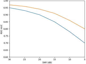
Fig. 3Noise robustness by integrated risk

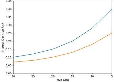
It should be emphasized that, for a fixed scoring function, the choice of the decision threshold does not change ROC-AUC, which measures only the ranking quality of the scores. The ROC-AUC differences in Fig. 2 and Table 1 are therefore attributable to the hybrid feature representation (CNN embeddings fused with statistical features), whereas the contribution of the risk-based adaptive threshold manifests itself in the risk-oriented metrics (Fig. 3) and in the position of the operating point (Figs. 4 and 5).

Fig. 3 shows the dependence of the integrated decision error (Bayesian risk) on the noise level. Unlike ROC-AUC metrics, risk directly accounts for the asymmetry in the error costs of C_FN and C_FP. The proposed method ensures minimal risk over a wide SNR range, which is critical for predictive diagnostics. At low SNR (5 dB), the risk for the baseline model increases by 4 times, while for the proposed model it increases by 2.5 times. Even at 5 dB, the risk remains lower than that of the baseline models.

Fig. 4ROC curves of the compared models with the isorisk tangency at the optimal operating point

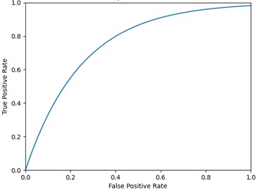
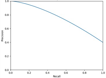
Fig. 5Precision-recall analysis

5.1. Computational complexity and real-time feasibility

One of the key requirements for intelligent predictive diagnostic systems is the ability to operate in near-real-time. This is particularly important for bearing vibration monitoring, where the sampling frequency can reach tens of kilohertz, and defect detection must be made with minimal latency. The per-window inference cost of the proposed architecture consists of three components. The cost of the CNN encoder is the sum over its layers of the multiply-accumulate (MAC) operations of the convolutions, $O\left({\mathrm{\Sigma }}_l{K}_l^2{C}_{l-1}{C}_l{H}_l{W}_l\right)$, where $K_l$ is the kernel size, $C_{l-1}$ and $C_l$ are the numbers of input and output channels, and $H_l\times W_l$ is the feature-map size of layer $l$; for the architecture specified in Section 4.1 this amounts to ≈ 10⁷ MAC per window. The cost of the gradient-boosting tabular block is $O\left(T·D\right)$ comparisons per window ($T=$ 200 trees of depth $D=$ 4, i.e., at most 800 comparisons). The risk-based decision layer reduces at run time to a single comparison of the calibrated score with the threshold, i.e., $O\left(1\right)$; the construction of the ROC curve and the selection of the operating threshold are performed offline on $N$ validation scores in $O\left(N\mathrm{l}\mathrm{o}\mathrm{g}N\right)$.

The resulting per-window latency budget is:

At the sampling rate of 12 kHz used in the experiments, a new 2048-sample window with 50 % overlap becomes available every 1024 samples, i.e., approximately every 85 ms, which corresponds to a decision-update rate of ≈11.7 Hz. The total per-window processing time, including preprocessing, feature extraction, inference of both blocks and the $O\left(1\right)$ threshold decision, is about 20 ms (see the timing breakdown in the engineering interpretation below), which leaves a real-time margin of more than a factor of four. The training procedure uses the Adam optimizer [29]; the deployment requirements are consistent with those discussed for intelligent fault diagnosis systems in [16].

5.2. Noise robustness analysis

As SNR decreases, quality metrics degrade. However, the risk-based mechanism demonstrates a slower increase in the integrated risk. From a theoretical perspective, robustness is due to the fact that the optimal threshold adapts to changes in feature distribution densities [6].

5.3. Resilience to distributional shift

The problem of distributional shift has been extensively studied in [17, 18]. Distributional shift is formalized as:

The divergence $D_{KL}\left(P_{train}\parallel P_{test}\right)$, estimated in the score space as described in Section 3.4, is used for shift detection; when the threshold τ is exceeded, the decision threshold is recalculated according to Eqs. (17) and (19). Under the assumptions of Proposition 1, the induced risk deviation is bounded by Eq. (20), which ensures Lipschitz stability of the risk functional with respect to bounded perturbations of the operating characteristics. For larger shifts the bound becomes loose, and the guarantee should be regarded as a worst-case statement rather than an empirical performance claim.

Table 1 shows the decrease in ROC-AUC with changes in operating conditions (load, rotation speed, sensor, mount). The proposed approach demonstrates a smaller loss in AUC due to hybrid features and a risk-based thresholding mechanism.

Table 2 shows the sensitivity of the integral risk to a systematic deviation of the probability estimates by $\epsilon$. The behaviour is non-monotonic: at small calibration errors ($\epsilon =$ 0.01 and $\epsilon =$ 0.05) the fixed-threshold baseline exhibits a smaller absolute risk deviation, and the advantage of the proposed method appears only at the largest miscalibration level ($\epsilon =$ 0.10), where the adaptive threshold partially compensates the displacement of the score distribution. The proposed method therefore cannot be claimed to have uniformly lower risk variability; Proposition 1 provides only a worst-case bound, which both strategies satisfy. Probability calibration is performed using the methods described in [24, 25]; a systematic experimental study of the observed non-monotonic behaviour under controlled calibration protocols is left for future work.

5.4. Engineering and applied interpretation

The proposed methodology reduces dependence on arbitrary thresholds, adapts to changing operating conditions, takes into account the economic consequences of errors, and is applicable to vibration engineering and seismic monitoring systems [31]. Under dynamic loads and environmental variability, the adaptive threshold allows maintaining a stable risk level, which is especially important for critical infrastructure assets.

The method integrates principles of control theory and dynamic-model identification [32], statistical decision making, and machine learning, forming a universal foundation for intelligent monitoring systems.

The average computational time, i.e., the average processing time of one window, is as follows:

– Preprocessing: ~3-5 ms.

– CNN inference: ~8-15 ms (IPC).

– Threshold recalculation: < 1 ms.

Resulting in $T_{total}\approx$ 20 ms. This enables near-real-time operation of the system.

5.5. Research limitations

The model was trained on a specific type of bearing. Degradation is possible at extremely low SNR (< 5 dB). Periodic recalibration is required.

Bearings are critical components of turbines, compressors, pumps, and electric motors. Early defect detection helps reduce accidents, minimize unscheduled shutdowns, and implement predictive maintenance.