Abstract
Digital Twin research in maintenance has matured around fault detection and diagnostics, yet the pathway from DT-derived risk estimates to defensible maintenance schedules remains underdeveloped. This paper proposes a four-stage, reliability-driven DT framework that specifies a particular method at each stage, rather than presenting the framework only as a concept. Stage 1 ranks assets through a Delphi-Analytic Hierarchy Process procedure that produces a Risk Priority Index integrating expert priority vectors with a percentile-based severity-occurrence rating. Stage 2 characterises system structure with a BowTie model that hybridises Fault Tree Analysis and Reliability Block Diagrams, yielding minimal cut sets, barrier effectiveness, and an explicit single-point-of-failure rule. Stage 3 combines a Cox proportional hazards model, with condition-monitoring covariates, and a cross-fitted residual-learning correction, yielding a hybrid linear predictor and a calibrated baseline cumulative hazard. Stage 4 converts the hazard outputs into decision quantities and optimises the preventive-maintenance interval and risk threshold via parametric simulation subject to an availability constraint. The framework is implemented as an offline, advisory Digital Twin with unidirectional data flow, calibrated and validated on synthetic and historical data using the C-index, Brier score, and expected calibration error. The contribution is a method-locked, decision-oriented architecture that links criticality, reliability structure, hazard modelling, and scheduling optimisation in a single, auditable workflow. The framework is conceptual at this stage; full empirical validation is the next step in the research programme.
Highlights
- Four-stage digital twin framework from asset criticality to schedule
- Delphi-AHP risk index ranks assets by expert consensus and percentile-based rating
- BowTie hybrid of FTA and RBD exposes minimal cut sets and single points of failure
- Cox model with residual learning yields a calibrated per-asset hazard
- Grid simulation sets PM interval and risk threshold under an availability limit
1. Introduction
Industrial assets fail in patterns that are rarely fully captured by either fixed-interval inspections or single-threshold alarms. Reactive repair is costly; calendar-based preventive maintenance discards remaining useful life; and threshold-based predictive maintenance can miss interactions between condition, operational load, and maintenance history. Digital Twin (DT) technology has been positioned as the route out of this trade-off, yet most published frameworks stop at fault detection or diagnostics and leave the link to a concrete maintenance schedule implicit [1]-[3]. This paper addresses that gap by proposing a four-stage, reliability-driven DT framework that fixes a specific method at each stage and shows how the outputs of one stage feed the next.
Three weaknesses recur across recent DT-for-maintenance literature. The first is a deterministic-stochastic gap. Twin models often rely on physics-based simulations or point estimates of remaining useful life, without quantifying uncertainty in the failure prediction itself [2], [4], [5]. The second is a risk-to-decision gap. Probabilistic risk outputs are produced but rarely converted into decision quantities such as the probability of failure inside a planning window, expected downtime, or cost per scheduling option [6]-[8]. The third is methodological inconsistency. Different studies pick different ranking schemes, reliability tools, and risk models, which limit scalability and prevent organisations from adopting a consistent risk-to-decision workflow [9]-[11].
These weaknesses are reinforced by shifts in research interests. Bibliometric reviews show that DT research has expanded rapidly under Industry 4.0 and now Industry 5.0, with strong activity in production planning and supply chain analysis [12]-[14]. Maintenance optimisation, by contrast, has received less structured attention. Predictive maintenance frameworks integrated with smart-manufacturing twins typically emphasise production schedules and treat preventive interventions as boundary conditions [15]. Where DT-based prognostics and health management have been proposed, the contribution is usually positioned at the monitoring layer rather than at the policy layer [16]-[18]. The result is a body of work that is rich in detection but thin on decision support.
The framework presented here is grounded in two foundational reference architectures. Grieves's three-dimensional model, physical asset, virtual asset, and the connection between them, defines what a DT is but stops short of specifying the maintenance logic that should sit atop it [19], [20]. Tao’s five-dimensional extension adds data and services as explicit components, thereby sharpening the implementation view while still leaving the maintenance-decision pipeline open [17]. Condition-based monitoring (CBM) principles in ISO 17359 [21] and reliability-modelling guidance in IEC 61025 [22] and BS EN 61078 [23] provide the missing technical grounding for diagnostics and reliability structure modelling. The contribution of this paper is to integrate these elements with a hazard-based risk model and a scheduling layer, thereby linking the four stages through explicit data products rather than narrative.
This paper expands on an earlier conceptual model proposed by the authors at International conference on Physical Asset Management and Data Science (PAMDaS 2025), in which the framework was outlined in terms of stage names. The present article specifies the method chosen at each stage, the decision rules that link the stages, and the validation strategy used to assess the framework against baseline maintenance practice. The contribution is therefore methodological rather than empirical: this is a concept paper in which the methodology is locked, while empirical validation is positioned as ongoing work.
Two research questions structure the contribution. (RQ1) Within an industrial DT setting, how can a systematic asset-ranking and reliability-analysis layer improve the identification of critical components and failure dependencies relative to single-method approaches? (RQ2) Within the same DT setting, how can a hazard-based risk model coupled with parametric simulation-based optimisation be configured to minimise downtime and total cost under realistic logistical constraints?
Section 2 sets out the proposed framework and the method selected at each stage. Section 3 sets out the variables and dataset requirements, and Section 4 concludes and outlines the validation roadmap.
2. Framework overview and method selection
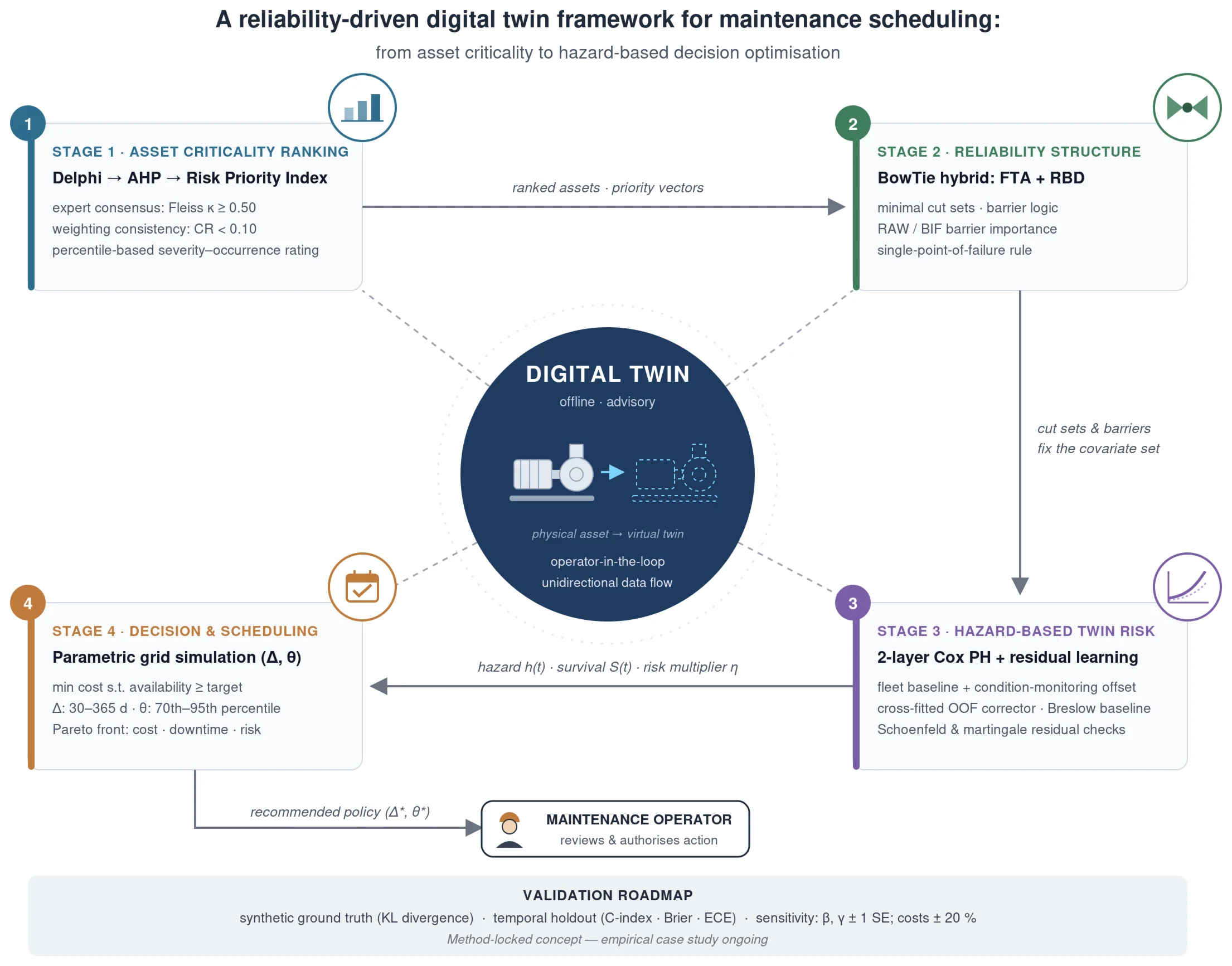
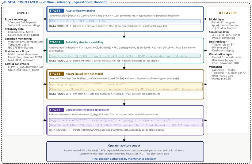
The framework is a four-stage analytical workflow embedded inside an offline, advisory DT (Fig. 1). Stage 1 (Asset Criticality Ranking) selects which assets should be modelled in detail. Stage 2 (Reliability Structure Modelling) characterises the failure logic of each critical asset, identifies dependencies, and evaluates the effectiveness of barriers. Stage 3 (Hazard-Based Twin Risk Model) converts condition-monitoring, operational, and maintenance covariates into a probabilistic hazard with uncertainty bounds. Stage 4 (Decision and Scheduling Optimisation) translates the hazard into decision quantities and finds the preventive-maintenance interval and risk threshold that minimise cost subject to an availability constraint. The DT layer hosts the analytical roadmap, ingests historical or synthetic data, runs offline calibration and what-if analyses, and presents recommendations to a maintenance operator.
Three properties bind the stages together. First, data products flow downstream: priority vectors from Stage 1 fix the scope of Stage 2; minimal cut sets and barrier diagrams from Stage 2 fix the covariate set for Stage 3; the hazard and survival functions from Stage 3 are the inputs to the optimisation in Stage 4. Second, every method is selected against a stated criterion of method-problem fit, not stylistic preference. Third, the DT operates as an operator-in-the-loop advisor, not as an autonomous controller: the framework produces recommendations; the operator authorises action.
Fig. 1Proposed reliability-driven DT framework with four analytical stages embedded in an offline, advisory DT, with the data products that link them
2.1. Stage 1 – asset criticality ranking (Delphi-AHP-RPI)
The first stage determines which assets justify deeper modelling. The chosen method is a three-step procedure that integrates qualitative expert elicitation, a quantitative weighting model, and a percentile-based risk index. The fit is deliberate: criticality decisions in industrial maintenance are driven by both expert tacit knowledge and quantitative trade-offs, and no single method captures both. Fig. 2 summarises the three-step Delphi-AHP-RPI workflow.
Step 1a uses a Delphi study to elicit and rank candidate criteria. A panel of ten experts is recruited through purposive and snowball sampling, with each expert holding at least five years of relevant maintenance or asset management experience, in line with CREDES guidance recommending panel sizes between 10 and 18 [24]. Experts complete a semi-structured questionnaire that maps sub-criteria, for instance, Average Annual Failure Rate (AAFR), Downtime Per Failure (DPF), and Replacement Cost (RC), onto the nine main criteria proposed by Jasiulewicz-Kaczmarek et al. [25]. The decision rule is that Fleiss’s kappa is at least 0.50 across criteria, with up to three rounds of feedback before the most frequently selected criteria are accepted by a majority. A preliminary correlation matrix prunes redundant sub-criteria with correlations above an 80 % threshold to avoid double-counting.
Step 1b applies the Analytic Hierarchy Process (AHP) to convert expert judgements into priority vectors [26]. Pairwise comparisons use Saaty’s 1-9 intensity scale across a four-level hierarchy: goal, main criteria, sub-criteria, and asset alternatives. The number of pairwise judgements per matrix is /2, with n the number of compared elements. For each pairwise matrix, the priority vector is computed by column normalisation, row summation, and division by the number of columns; the maximum eigenvalue, , is obtained by multiplying the original matrix by the priority vector and dividing element-wise. Internal consistency is enforced through the Consistency Index and Consistency Ratio, with CR < 0.10 as the acceptance threshold. The geometric mean is used to aggregate the 10 experts’ ratings because it preserves the reciprocal nature of the Saaty scale:
Fig. 2Stage 1 asset criticality ranking. Delphi-AHP-RPI: expert elicitation
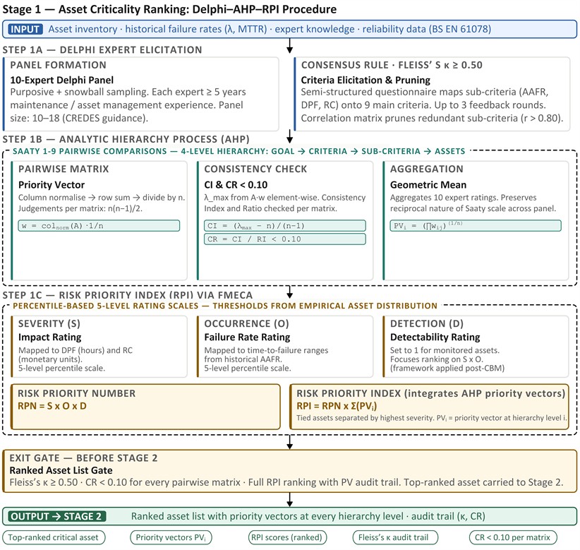
Step 1c integrates AHP weights with Failure Mode, Effects, and Criticality Analysis (FMECA) into a Risk Priority Index (RPI). Severity (S), Occurrence (O), and Detection (D) are scored on percentile-based 5-level rating scales drawn from the empirical distribution of each criterion in the asset population, so that thresholds reflect the data rather than analyst intuition. Occurrence is mapped to time-to-failure ranges; severity is mapped to criterion values, such as DPF (in hours) and RC (in monetary units). Detection is set to 1 when the framework is applied to assets already being monitored, which focuses the ranking on severity and occurrence. The Risk Priority Number and Risk Priority Index are:
where is the priority vector at hierarchy level . Tied assets are separated by the highest severity rating. The output of Stage 1 is a ranked asset list with explicit priority vectors at every hierarchy level, an audit trail of expert agreement (Fleiss’s kappa), and a CR < 0.10 check for every pairwise matrix. The asset at the top of the RPI ranking is carried into Stage 2.
2.2. Stage 2 – reliability structure modelling (BowTie hybrid)
Stage 2 explains how the failure logic of each critical asset is modelled using BowTie analysis. BowTie illustrates how threats lead to a top event (on the fault tree's left side) and how consequences develop (on the event tree’s right side). Fault Tree Analysis (FTA) determines the logical combinations of basic events that trigger the top event; BowTie adds preventive and mitigative barriers on top. Reliability Block Diagram (RBD) concepts organise barriers in series, parallel, or k-out-of-n arrangements, but BowTie applies a defence-in-depth principle: if any barrier succeeds, the process halts. This hybrid approach complies with IEC 61025 [22] and BS EN 61078 [23], offering a decision-focused perspective that connects causes, barriers, and outcomes. Fig. 3 summarises the three-step BowTie hybrid workflow.
Fig. 3Stage 2 reliability structure modelling workflow using a BowTie hybrid
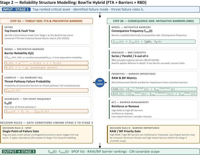
Step 2a involves three steps. First, the top event is identified based on the critical failure mode identified in Stage 1, and a Fault Tree Analysis (FTA) is constructed. Threat failure rates are derived from historical data.
Step 2b lists preventive barriers. Each barrier’s metrics, including probability of failure on demand (PFDavg), failure per hour (PFH), human-error probability (HEP), or conditional probability (), are transformed into a time-dependent reliability . For a barrier with a constant failure rate , this relationship is given by:
giving a failure probability:
For a constant error or conditional probability (), the reliability is written as:
The probability that all preventive barriers on a threat pathway fail is written as:
Summing over threats yields the top-event frequency:
Step 2c models mitigative barriers in the same way. The consequence frequency is expressed as:
Two decision rules link Stage 2 to Stage 3. A single-point-of-failure (SPOF) rule flags any basic event whose unmitigated occurrence triggers the top event; such SPOFs are either reinforced with redundancy or escalated to Stage 3. A barrier-importance rule uses Risk Achievement Worth (RAW) and Barrier Importance Factor (BIF) to prioritise barriers, which are written as:
High-RAW or high-BIF barriers are reinforced or improved; low-impact barriers may be removed. The output is a list of dominant threats, critical components and high-impact barriers; these feed the hazard-based twin risk model in Stage 3.
2.3. Stage 3 – hazard-based twin risk model (Cox PH with residual learning)
Stage 3 estimates the probabilistic risk influencing the schedule. It uses a two-layer Cox proportional hazards (PH) model with residual-learning correction, structured in three stages: a fleet baseline, a condition-monitoring (CM) offset, and a cross-fitted machine-learning corrector. The model fitting is explicit. Cox PH is semi-parametric, manages right-censored lifetimes, and provides interpretable hazard ratios, which are important for transparency in maintenance decision-making [27], [28]. The two-layer split preserves industrial context (the full fleet) while learning from the smaller monitored subset where covariates are recorded. Residual learning addresses the standard limitation of linear Cox: nonlinear and interaction effects in covariates that the linear predictor cannot capture [28]. Fig. 4 summarises the three-step Cox PH and residual-learning workflow.
Step 3b expresses the base hazard for an asset with covariate vector is:
where is the baseline hazard, and beta is the vector of log-hazard ratios. In the proposed framework, this is extended into a two-layer formulation. The fleet layer is fitted on units (e.g. 72 in the authors’ pilot dataset) with fleet-wide covariates :
The CM layer is fitted on the monitored subset (typically a fraction of ) using as a fixed offset, so that fleet-level information is preserved while the linear predictor learns from the monitored covariates :
A residual corrector is then trained out-of-fold (OOF) on the monitored subset in Step 3c. The OOF protocol partitions the monitored subset into -folds, fits the CM-layer Cox on folds, generates residuals on the held-out fold, and trains a non-linear learner, for example, a gradient-boosted tree, to predict the residuals on the held-out fold. The final deployment model refits Cox jointly on beta and gamma, with computed from the trained learner:
The baseline cumulative hazard is estimated by the Breslow estimator:
where:
and is the number of events at time ( and is the at-risk indicator. Covariates are -standardised before fitting (); and are stored as part of the deployment artefact, so that incoming sensor values are scaled consistently inside the DT.
Two assumption checks, in Step 3d, are mandatory before the model is exported. The proportional-hazards assumption is tested using Schoenfeld residuals [29] over time and by assessing the linearity of the log-cumulative hazard. Martingale residuals are inspected for systematic dependence on covariates [30]. If either check fails on a covariate, either a stratified-baseline Cox is fitted, or the residual-learning correction is enabled to absorb the non-linearity. The data leakage rule is firm: the residual target used to train z must always be out-of-fold, and the final is refitted on the full monitored subset only after OOF predictions are in place.
Fig. 4Stage 3 hazard-based twin risk model workflow
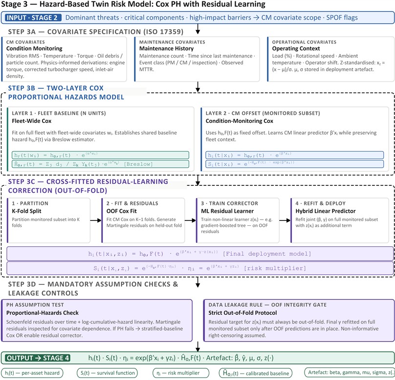
Variable specification follows ISO 17359 indicators [21]. Condition-monitoring covariates include vibration RMS, temperature, torque, and oil debris or particle count; physics-informed derivations (engine torque from power and speed; corrected turbocharger speed using inlet-air temperature; inlet-air density from absolute pressure and temperature) are available as engineered covariates when sensor coverage permits. Maintenance covariates include maintenance count, time since last maintenance, event class (preventive, corrective, inspection), and observed MTTR. Operational covariates include load, rotational speed, ambient temperature, and operator shift. Censoring is treated as right-censored and assumed non-informative conditional on covariates; the lifecycle outcome is binary (failure vs censored), and the post-maintenance state is treated as as-good-as-new for the bearing-replacement scenario considered in the pilot.
The output of Stage 3 is a per-asset hazard , survival , risk multiplier , and a calibrated . These are the inputs to Stage 4.
2.4. Stage 4 – decision and scheduling optimisation (parametric simulation)
Stage 4 converts the hazard into decision-ready maintenance quantities, including rolling-window failure probability, expected downtime, cost, and availability. The first implementation is a parametric simulation over a two-dimensional decision grid (preventive-interval and risk-threshold ). For each candidate (), the simulation applies trigger logic, computes cost, downtime, failure-risk and availability outcomes, and identifies the best feasible policy under an availability constraint. This paper opts for a grid-based simulation as the first implementation because the decision space is low-dimensional and directly auditable. A Pareto front is then extracted to support a decision maker who must trade cost, downtime, and risk. Fig. 5 summarises the three-step decision and scheduling-optimisation workflow.
Fig. 5Stage 4 decision and scheduling optimisation workflow
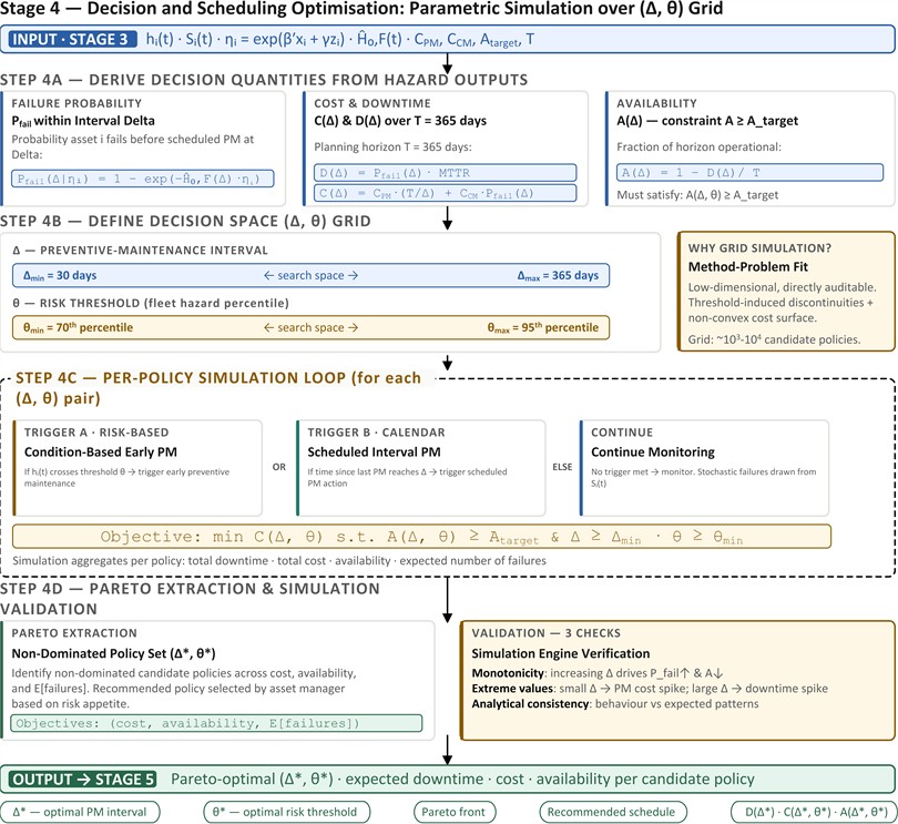
In Step 4a, the decision quantities are derived from the hazard and survival functions of Stage 3. The probability of failure inside an interval for asset is:
Expected downtime, total cost, and availability are:
where is the analysis horizon (typically 365 days), is the cost per preventive action, and is the cost per corrective action. The optimisation is:
The decision space is searched over in [30, 365] days and between the 70th and 95th percentile of the fleet hazard distribution in Step 4b. The combined grid yields roughly 103-104 candidate policies. For each (, ) pair in Step 4c, the simulation engine evaluates the asset over the analysis horizon: if crosses , an early preventive intervention is triggered; if the time since the last preventive action reaches , a scheduled preventive action is triggered; otherwise, monitoring continues. Stochastic failure events are drawn from . The simulation aggregates total downtime, total cost, and availability per policy.
Pareto extraction, in Step 4d, can be applied after the grid simulation to identify the non-dominated candidate policies (, ) across cost, availability, and expected number of failures. The recommended policy () is then selected by the asset manager based on risk appetite. Validation of the simulation engine is enforced through three checks: monotonicity (increasing within the tested grid drives and downtime upward and availability downward), extreme values (very small must produce a PM cost spike; very large must produce a downtime spike), and analytical consistency checks against expected behaviour.
2.5. Stage 5 – DT integration and offline validation
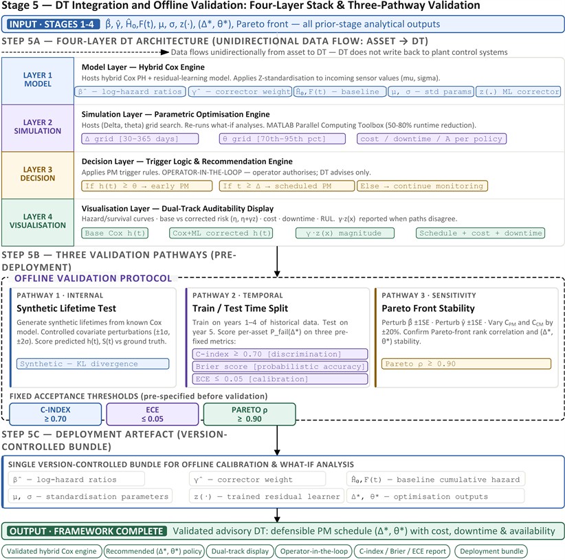
The DT prototype is implemented as a four-layer stack, as outlined in Step 5a, with unidirectional data flow across the model, simulation, decision, and visualisation layers. The model layer hosts the hybrid Cox engine and the standardisation parameters. The simulation layer hosts the parametric optimisation. The decision layer applies the trigger logic and emits the recommendation. The visualisation layer presents hazard curves, survival curves, base versus corrected risk scores, and the recommended schedule with cost and downtime estimates. A dual-track display, based on Cox versus Cox with residual correction, is provided to support auditability: when the two paths disagree, the magnitude of is reported to expose the contribution of the corrector. Fig. 6 summarises the three-step DT integration, calibration, and validation workflow.
The DT operates offline as an advisory tool. Implementing real-time streaming is planned for future development. Data flows only from the asset to the DT, with no feedback to plant control systems. This design choice maintains the framework’s auditability and supports operator-in-the-loop decision-making, while also isolating the analytical workflow from potential control-loop interactions.
Three validation pathways are used in Step 5b before deployment. Internal validation generates synthetic asset lifetimes from a known Cox model with controlled covariate perturbations (, ); the predicted hazard and survival are scored against the synthetic ground truth using the Kullback-Leibler divergence [31]. Temporal validation trains the DT on years 1-4 of historical data and tests on year 5, scoring per-asset using Harrell’s C-index, the Brier score, and the Expected Calibration Error (ECE) [32]-[34]. Sensitivity analysis perturbs the final by ±1 SE, perturbs final similarly, and varies and by ±20 % to test the stability of the Pareto front and of the recommended () policy.
Fig. 6Stage 5 DT integration and offline validation workflow
3. Variables and dataset requirements
The minimum dataset to operationalise the framework comprises four blocks. Survival fields: asset identifier, install or last-replacement date, observation end date, time-to-event in days, and the binary event indicator (1 = failure, 0 = censored). CM covariates aligned to ISO 17359 [21]: vibration RMS, temperature, torque, and oil debris/particle count. Maintenance covariates: maintenance count, time since last maintenance, event class, and observed MTTR. Operational covariates: load (% or power proxy), rotational speed, ambient temperature, and operator shift. Scheduling-realism variables, spare lead time, crew availability, spare-inventory policy, and economic variables, , , downtime cost per hour, and availability target are required for Stage 4. The full set is shown in Table 1.
4. Conclusions
This paper has expanded the four-stage DT-for-maintenance framework introduced at PAMDaS 2025 from a concept-level outline into a method-locked architecture. At Stage 1, asset criticality is fixed through a Delphi-AHP-RPI procedure that combines expert agreement (Fleiss’s kappa ≥ 0.50, geometric-mean aggregation), a consistency-checked weighting model (CR < 0.10), and a percentile-based RPI. At Stage 2, the system structure is fixed using a BowTie hybrid that employs FTA for causes, RBD for system reliability, and explicit barrier modelling on the consequence side. At Stage 3, the twin risk model is fixed as a two-layer Cox proportional hazards model with a cross-fitted residual-learning correction, giving a hybrid linear predictor and a Breslow-estimated baseline cumulative hazard. At Stage 4, the scheduling problem is formulated as a parametric simulation over preventive interval and risk threshold with a cost objective and an availability constraint, and the Pareto front is presented to the decision maker.
Table 1Minimum dataset specification for the proposed framework
Survival fields | Asset ID; install/last replacement date; observation end date; time-to-event (days); event indicator (1 = failure, 0 = right-censored) |
Condition-monitoring covariates | Vibration RMS; temperature (Celsius); torque (Nm); oil debris/particle count (ISO 17359 indicators) |
Maintenance covariates | Maintenance count; time since last maintenance (days); event class (PM/CM/inspection); observed MTTR |
Operational covariates | Load (%) or power proxy; rotational speed (RPM); ambient temperature (Celsius); operator shift/team |
Scheduling and economic variables | Spare lead time (days); crew availability; ; ; downtime cost per hour; availability target |
Three properties distinguish the framework from existing DT-for-maintenance proposals. The first is method-problem fit at every stage rather than a generic stack of fashionable techniques. The second is explicit data products linking the stages, so that priority vectors, minimal cut sets, hazard functions, and optimal policies are propagated rather than re-derived. The third is auditability: every method exposes a decision rule (CR threshold, SPOF rule, PH-assumption check, dual-track Cox-vs-Cox-plus-ML display, Pareto front), so that a maintenance team can challenge any individual recommendation.
The contribution is conceptual at this stage. The framework specifies methods, decision rules, and validation thresholds, but the empirical case study is ongoing. The framework is offered as a defensible, decision-oriented starting point rather than as a final word, and it is intended to be tested against the realities of industrial maintenance rather than only against published benchmarks.
References
-
H. Liu, M. Xia, D. Williams, J. Sun, and H. Yan, “Digital twin-driven machine condition monitoring: a literature review,” Journal of Sensors, Vol. 2022, pp. 1–13, Jul. 2022, https://doi.org/10.1155/2022/6129995
-
A. Rasheed, O. San, and T. Kvamsdal, “Digital twin: values, challenges and enablers from a modeling perspective,” IEEE Access, Vol. 8, pp. 21980–22012, Jan. 2020, https://doi.org/10.1109/access.2020.2970143
-
R. van Dinter, B. Tekinerdogan, and C. Catal, “Predictive maintenance using digital twins: a systematic literature review,” Information and Software Technology, Vol. 151, p. 107008, Nov. 2022, https://doi.org/10.1016/j.infsof.2022.107008
-
X. Qiao, V. L. Jauw, L. C. Seong, and T. Banda, “Advances and limitations in machine learning approaches applied to remaining useful life predictions: a critical review,” The International Journal of Advanced Manufacturing Technology, Vol. 133, No. 9-10, pp. 4059–4076, Jun. 2024, https://doi.org/10.1007/s00170-024-14000-0
-
S. Sankararaman, “Significance, interpretation, and quantification of uncertainty in prognostics and remaining useful life prediction,” Mechanical Systems and Signal Processing, Vol. 52-53, pp. 228–247, Feb. 2015, https://doi.org/10.1016/j.ymssp.2014.05.029
-
F. I. Khan and M. M. Haddara, “Risk-based maintenance (RBM): a quantitative approach for maintenance/inspection scheduling and planning,” Journal of Loss Prevention in the Process Industries, Vol. 16, No. 6, pp. 561–573, Nov. 2003, https://doi.org/10.1016/j.jlp.2003.08.011
-
E. Leo, S. Engell, and I. E. Grossmann, “Condition-based maintenance optimization via stochastic programming with endogenous uncertainty,” Computers and Chemical Engineering, Vol. 156, p. 107550, 2022, https://doi.org/10.1016/j.compchemeng.2021.107550
-
B. Coutinho, M. Moreira, E. Pereira, and G. Gonçalves, “Survival analysis-based system for predictive maintenance optimization,” SN Computer Science, Vol. 6, No. 7, Aug. 2025, https://doi.org/10.1007/s42979-025-04291-9
-
B. Xiao, J. Zhong, X. Bao, L. Chen, J. Bao, and Y. Zheng, “Digital twin-driven prognostics and health management for industrial assets,” Scientific Reports, Vol. 14, No. 1, Jun. 2024, https://doi.org/10.1038/s41598-024-63990-0
-
G. Pronost, F. Mayer, M. Camargo, and L. Dupont, “Digital twins along the product lifecycle: a systematic literature review of applications in manufacturing,” Digital Twin, Vol. 1, No. 2, Dec. 2024, https://doi.org/10.12688/digitaltwin.17807.2
-
M.-E. Iliuţă, M.-A. Moisescu, E. Pop, A.-D. Ionita, S.-I. Caramihai, and T.-C. Mitulescu, “Digital Twin-A review of the evolution from concept to technology and its analytical perspectives on applications in various fields,” Applied Sciences, Vol. 14, No. 13, p. 5454, 2024, https://doi.org/10.3390/app14135454
-
W. S. Lam, W. H. Lam, and P. F. Lee, “A bibliometric analysis of digital twin in the supply chain,” Mathematics, Vol. 11, No. 15, p. 3350, Jul. 2023, https://doi.org/10.3390/math11153350
-
V. Warke, S. Kumar, A. Bongale, and K. Kotecha, “Sustainable development of smart manufacturing driven by the digital twin framework: a statistical analysis,” Sustainability, Vol. 13, No. 18, p. 10139, Sep. 2021, https://doi.org/10.3390/su131810139
-
L. Gao, S. Li, and H. Guo, “Visualization and analysis of research areas and hot topics in the field of digital twins,” IEEE Access, Vol. 12, pp. 26897–26904, Jan. 2024, https://doi.org/10.1109/access.2024.3365291
-
Q. Feng et al., “Multi-level predictive maintenance of smart manufacturing systems driven by digital twin: a matheuristics approach,” Journal of Manufacturing Systems, Vol. 68, pp. 443–454, Jun. 2023, https://doi.org/10.1016/j.jmsy.2023.05.004
-
M. Molęda, B. Małysiak-Mrozek, W. Ding, V. Sunderam, and D. Mrozek, “From corrective to predictive maintenance-a review of maintenance approaches for the power industry,” Sensors, Vol. 23, No. 13, p. 5970, 2023, https://doi.org/10.3390/s23135970
-
F. Tao, M. Zhang, Y. Liu, and A. Y. C. Nee, “Digital twin driven prognostics and health management for complex equipment,” CIRP Annals, Vol. 67, No. 1, pp. 169–172, Jan. 2018, https://doi.org/10.1016/j.cirp.2018.04.055
-
Y. Lu, C. Liu, K. I.-K. Wang, H. Huang, and X. Xu, “Digital twin-driven smart manufacturing: connotation, reference model, applications and research issues,” Robotics and Computer-Integrated Manufacturing, Vol. 61, p. 101837, Feb. 2020, https://doi.org/10.1016/j.rcim.2019.101837
-
M. Grieves, “Digital twin: manufacturing excellence through virtual factory replication,” Florida Institute of Technology, 2014.
-
M. Grieves and J. Vickers, “Digital twin: mitigating unpredictable, undesirable emergent behavior in complex systems,” in Transdisciplinary Perspectives on Complex Systems, Cham: Springer International Publishing, 2016, pp. 85–113, https://doi.org/10.1007/978-3-319-38756-7_4
-
“Condition Monitoring and Diagnostics of Machines – General Guidelines,” ISO: 17359, Geneva, Switzerland, 2018.
-
“IEC 61025: Fault Tree Analysis (FTA),” International Electrotechnical Commission, Geneva, Switzerland, 2006.
-
“BS EN 61078: Reliability Block Diagrams,” British Standards Institution, London, UK, 2016.
-
E. E. Odjegba, G. Oluwasanya, O. A. Idowu, and O. B. Shittu, “Failure mode effects and criticality analysis of water supply systems’ risks: path to water resources planning and policy,” Water and Environment Journal, Vol. 37, No. 1, pp. 114–125, 2023, https://doi.org/10.1111/wej.12822
-
M. Jasiulewicz-Kaczmarek, K. Antosz, P. Żywica, D. Mazurkiewicz, B. Sun, and Y. Ren, “Framework of machine criticality assessment with criteria interactions,” Eksploatacja I Niezawodność – Maintenance and Reliability, Vol. 23, No. 2, pp. 207–220, Jun. 2021, https://doi.org/10.17531/ein.2021.2.1
-
T. L. Saaty, “How to make a decision: the analytic hierarchy process,” European Journal of Operational Research, Vol. 48, No. 1, pp. 9–26, Sep. 1990, https://doi.org/10.1016/0377-2217(90)90057-i
-
D. R. Cox, “Regression models and life-tables,” Journal of the Royal Statistical Society Series B: Statistical Methodology, Vol. 34, No. 2, pp. 187–202, 1972, https://doi.org/10.1111/j.2517-6161.1972.tb00899.x
-
D. R. Godoy, C. Mavrakis, R. Mena, F. Kristjanpoller, and P. Viveros, “An advanced framework for predictive maintenance decisions: integrating the proportional hazards model and machine learning techniques under CBM multi-covariate scenarios,” Applied Sciences, Vol. 14, No. 13, p. 5514, Jun. 2024, https://doi.org/10.3390/app14135514
-
P. M. Grambsch and T. M. Therneau, “Proportional hazards tests and diagnostics based on weighted residuals,” Biometrika, Vol. 81, No. 3, pp. 515–526, Jan. 1994, https://doi.org/10.1093/biomet/81.3.515
-
D. Y. Lin, L. J. Wei, and Z. Ying, “Checking the Cox model with cumulative sums of martingale-based residuals,” Biometrika, Vol. 80, No. 3, pp. 557–572, Jan. 1993, https://doi.org/10.1093/biomet/80.3.557
-
S. Kullback and R. A. Leibler, “On information and sufficiency,” The Annals of Mathematical Statistics, Vol. 22, No. 1, pp. 79–86, Mar. 1951, https://doi.org/10.1214/aoms/1177729694
-
Frank E. Harrell Jr, et al., “Evaluating the yield of medical tests,” JAMA: the Journal of the American Medical Association, Vol. 247, No. 18, p. 2543-2546, 1982, https://doi.org/10.1001/jama.1982.03320430047030
-
T. A. Gerds and M. Schumacher, “Consistent estimation of the expected Brier score in general survival models with right-censored event times,” Biometrical Journal, Vol. 48, No. 6, pp. 1029–1040, 2006, https://doi.org/10.1002/bimj.200610301
-
C. Guo, G. Pleiss, Y. Sun, and K. Q. Weinberger, “On calibration of modern neural networks,” in 34th International Conference on Machine Learning, pp. 1321–1330, 2017.
About this article

The authors acknowledge the supervision and methodological guidance provided within the School of Engineering, The University of Manchester, and the Alliance Manchester Business School. No external funding was received specifically for the work reported in this paper.
This is a methodology paper; no new experimental dataset is reported. The synthetic and historical datasets used to develop and pilot-test the framework are available from the corresponding author on reasonable request.
M. A. Amiruddin: conceptualisation, methodology, formal analysis, software, visualisation, writing-original draft preparation. K. A. Papadopoulou: conceptualisation, methodology, supervision, writing-review and editing.
The authors declare that they have no conflict of interest.
This research did not involve human or animal subjects; therefore, an ethics approval was not required.

