Abstract
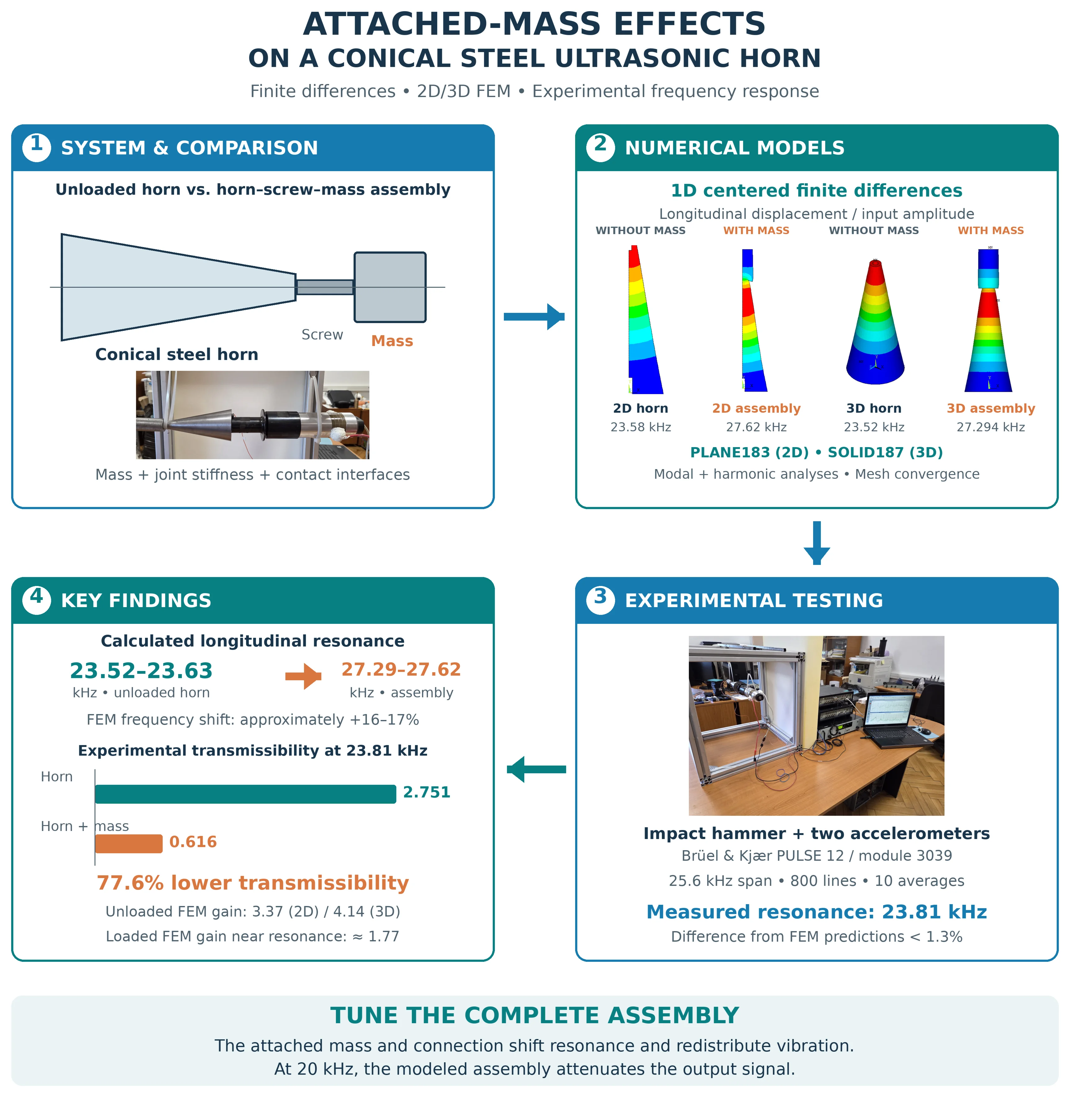
This study evaluates the effects of an attached mass on the dynamic response of a conical steel ultrasonic horn using a centered finite-difference scheme, axisymmetric 2D and full 3D ANSYS FEM models, and impact-hammer FRF testing. Modal and harmonic analyses compare the unloaded horn with the assembly comprising the screw, contacts, and mass. The added components shift the longitudinal resonance and redistribute displacement amplitude, producing detuning and modal-response redistribution rather than uniform attenuation.
Highlights
- Agreement between FEM models: the longitudinal frequencies predicted by the 2D and 3D models differ by only 0.25%.
- Resonance shift caused by the attached mass: the horn–screw–mass assembly exhibits a calculated resonance of 27.3–27.6 kHz, approximately 16–17% above that of the unloaded horn.
- Experimental reduction in transmissibility: at 23.81 kHz, the attached mass reduces transmissibility by 77.6%, highlighting the need to tune the complete ultrasonic assembly.
1. Introduction
Ultrasonic systems are widely used in machining, welding, cutting, cleaning, imaging, and surgery. They typically comprise a high-frequency generator and amplifier, an electromechanical transducer, and an ultrasonic horn. In loaded-horn models, the attached component is generally represented as terminal mechanical impedance rather than an ideal point mass. It may be modeled as a concentrated mass (e.g., using ANSYS MASS21), a mass-spring-damper system, a finite-element solid, or an elastic workpiece in contact with the horn. Although an ideal terminal mass usually lowers the natural frequency, a real horn-screw-mass assembly may increase or decrease it because the joint modifies the system’s mass, stiffness, effective length, and boundary conditions. Therefore, accurate models should include joint stiffness and damping and be validated through modal, harmonic, and experimental frequency-response analyses [1-4].
2. Types of ultrasonic horns
2.1. Mathematical description of ultrasonic wave propagation
An ultrasonic horn generally has two end faces with different cross-sectional areas. The one-dimensional model used to describe longitudinal-wave propagation through an ultrasonic horn is given in [5]:
where is the cross-sectional area variation, is the longitudinal wave velocity in the material, and is the axial displacement field, that depends on position and time .
2.2. Types of ultrasonic horns
For most industrial horns, the cross-section is circular and the diameter follows a prescribed variation law along the horn axis. This profile affects the displacement-amplification ratio, stress distribution, resonant behavior, and manufacturability. These profiles remain common because they combine predictable dynamic behavior with relatively straightforward manufacturing. The most commonly used ultrasonic horns are [6]-[8]:
1) Stepped ultrasonic horn – consists of two axial sections with different constant diameters.
2) Conical horn – provides smooth stress distribution and efficient force transmission useful for high-force machining and welding.
3) Exponential ultrasonic horn – the diameter profile decreases according to an exponential.
4) Catenoidal horn – smooth hyperbolic-cosine profile that enables high-force transmission, moderate amplitude gain, and improved fatigue life.
Horn selection and shape optimization must balance requirements such as displacement gain, force transmission, stress level, and fatigue life [9-11].
3. Models of the ultrasonic system
Previous studies have investigated dynamic behavior [12], [13]. This paper examines modeling approaches for analyzing the dynamic behavior of an ultrasonic system with an attached mass. The following methods were considered: the centered finite-difference method and 2D and 3D finite element analyses performed using ANSYS APDL.
3.1. Finite difference method
For the finite-difference model, a centered-difference scheme was applied to the propagation equation defined by Eq. (1), written for the spatial component of the solution to Webster’s equation. Applying the centered finite-difference method yields the following spatial equation:
where is the coefficient describing the geometric variation of the circular cross-section along the longitudinal axis.
Applying Eq. (2) at all axial nodes requires two boundary conditions: an input amplitude at the horn’s maximum cross-section and dynamic equilibrium at its output end, given by the following equation:
Assuming a harmonic ultrasonic signal, , and applying the centered finite-difference method, Eq. (3) becomes:
Eq. (3) and (4), combined with the prescribed input amplitude , yield a linear system of equations. In matrix form, the tridiagonal coefficient matrix contains the terms associated with the neighboring amplitudes , , and , while the right-hand-side is zero except for the component corresponding to .
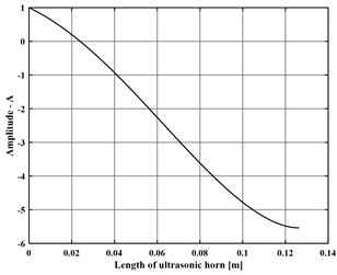
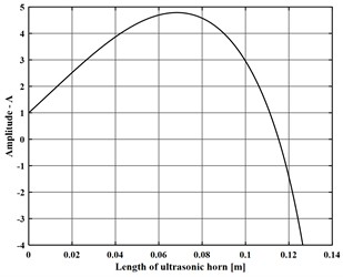
A MATLAB® 2023b [14] script implementing the centered finite-difference method simulated the horn response both without and with the experimentally tested attached mass (Fig. 1). The axial amplitudes were normalized by the input amplitude to determine the amplification factor.
Fig. 1Variation in signal magnification along the longitudinal axis: a) without the attached mass; b) with the attached mass
a)
b)
3.2. The 2D FEM model
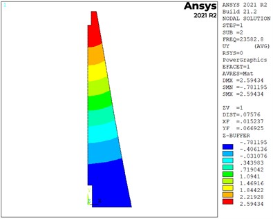
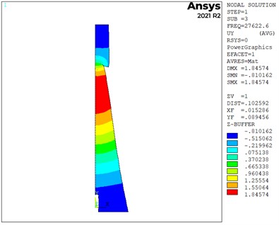
A computationally efficient 2D axisymmetric PLANE183 model captured the longitudinal and radial modes [15], with local refinement and mesh convergence assessed in Table 1. Harmonic analysis results are presented in Table 2. The calibrated PLANE183 2D model of the horn–screw–mass assembly showed attenuation at 20 kHz and approximately 1.77× amplification at its natural frequency (Fig. 2).
In general, the attached mass reduces the amplification ratio.
Table 1Natural frequencies for the 2D model
No. | Element length [m] | Nodes | Elements | Longitudinal natural frequency | Harmonic-analysis gain |
1. | 0.50e-3 | 30530 | 9977 | 23614.5 [Hz] | 3.3706 |
2. | 1.00e-3 | 7681 | 2460 | 23609.8 [Hz] | 3.3715 |
3. | 1.50e-3 | 3248 | 1015 | 23596.3 [Hz] | 3.3727 |
4. | 2.00e-3 | 1956 | 601 | 23582.8 [Hz] | 3.3746 |
Table 2Harmonic analysis – 2D assembly model
No. | Modal analysis | Harmonic-analysis gain analysis | ||||
Element length [m] | Nodes | Elements | Longitudinal natural frequency | Horn length at 20,000 Hz | Horn length calculated for 20,000 Hz | |
1. | 0.50e-3 | 38734 | 12718 | 27594.3 [Hz] | 0.5255 | 1.7874 |
2. | 1.00e-3 | 9708 | 3139 | 27603.2 [Hz] | 0.5217 | 1.7817 |
3. | 1.50e-3 | 3760 | 1189 | 27610.7 [Hz] | 0.5191 | 1.7788 |
4. | 2.00e-3 | 2283 | 712 | 27622.6 [Hz] | 0.5132 | 1.7676 |
3.3. The 3D finite element model
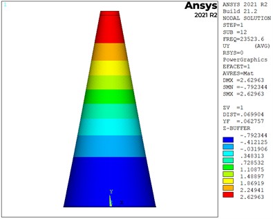
The 3D horn model was generated by revolving the 2D geometry and joining the volumes using VADD. SOLID187 elements were employed, with a refined 1 mm mesh near the holes and variable element sizes elsewhere. The 3D model was analyzed under free-free conditions using four, mesh sizes, while harmonic simulations at the first longitudinal natural frequency determined the signal amplification (Table 3).
A 4 mm element size provides nearly the same natural frequency as the 2 mm mesh, with a difference of only 0.0008 % and approximately 61 % fewer elements. A 6 mm mesh offers the best compromise between accuracy and computational cost, whereas coarser meshes of 8 mm produce increasingly noticeable deviations. Under free-free conditions, the horn exhibited an amplification ratio of approximately 4.14, with negligible mesh dependence. The 3D model was then extended to include the screw, contact interfaces, and attached mass, using calibrated component masses and locally refined meshes to determine the loaded natural frequencies (ultrasonic horn 1.231 kg, screw 0.002 kg, and attached mass 0.193 kg) (Table 4). The density assigned in ANSYS was calculated from the mass and volume of each component. All components were assumed to be made of steel, with a Young’s modulus of 210 GPa and a Poisson’s ratio of 0.3.
Fig. 2Mode shapes of the 2D models with the same element size (2 mm): a) modal analysis of the single ultrasonic horn at a natural frequency of 23,582.8 Hz; b) harmonic analysis of the assembly at a frequency of 27,622.6 Hz
a)
b)
Table 3Natural frequencies for the 3D model
No. | Element length [m] | No. of nodes | No. of elements | Longitudinal natural frequency [Hz] | Harmonic-analysis gain |
1. | 0.002 | 254076 | 177027 | 23523.6 | 4.1412 |
2. | 0.004 | 98389 | 65479 | 23523.8 | 4.1412 |
3. | 0.006 | 72015 | 46502 | 23525.2 | 4.1418 |
4. | 0.008 | 67088 | 43004 | 23526.4 | 4.1413 |
Table 4Natural frequencies – 3D model
No. | Modal analysis | Harmonic-analysis gain analysis | ||||
Element length [m] | No. of nodes | No. of elements | Longitudinal natural frequency | Case of initial considered frequency (20 kHz) | Reconsidered natural frequency | |
1. | 0.002 | 678373 | 492946 | 27322.7 [Hz] | 0.6312 | 1.7638 |
2. | 0.004 | 281792 | 203957 | 27324.1 [Hz] | 0.6312 | 1.7652 |
3. | 0.006 | 198809 | 143952 | 27319.0 [Hz] | 0.6309 | 1.7668 |
4. | 0.008 | 165494 | 120205 | 27307.8 [Hz] | 0.6301 | 1.7753 |
As shown in Table 4, the harmonic analysis indicated that the horn designed for 20 kHz attenuated the output signal, whereas adjusting its length to tune the horn to the assembly’s natural frequency produced nearly mesh-independent amplification.
4. Experimental analysis
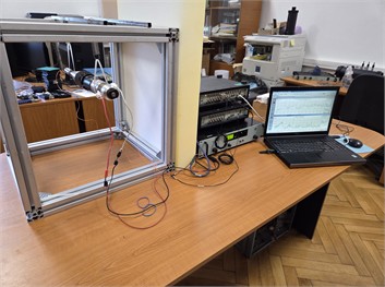
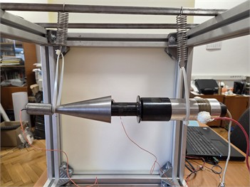
The experimental setup for identifying the natural frequencies of the conical horn and the complete ultrasonic system included the Brüel & Kjær PULSE 12 platform equipped with a 3039 module, two 4517-002 accelerometers (0.65 g; nominal range up to 20 kHz) and an 8206-003 aluminum-tipped impact hammer (Fig. 4). Data were processed using Brüel & Kjær software over a 25.6 kHz frequency span, with 800 spectral lines and 10 averages. The modal measurements were obtained from impacts applied in the longitudinal, transverse (radial), and vertical directions, with a coherence greater than 0.7 (Table 5).
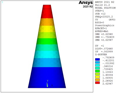
Fig. 3Mode shapes for 3D models considering two values of natural frequency: a) frequency of 23523.6 Hz (element length 2 mm); b) frequency of 23525.2 Hz (element length 6 mm)
a)
b)
Fig. 4The setup used for testing: a) the complete experimental system; b) the connection between the transducer, ultrasonic horn, and attached mass, with the accelerometers positioned at the measurement points
a)
b)
Table 5Natural frequencies of the ultrasonic horn determined experimentally using an impact hammer
No. | Impact hammer – modal frequency | Transmissibility horn | Transmissibility horn-attached mass | |||
Natural frequency [Hz] | Coherence [–] | Frequency [Hz] | Gain [-] | Frequency [Hz] | Gain [–] | |
1 | 20090 | 0.724 | 20090 | 0.955 | 20090 | 0.546 |
2 | 23810 | 0.838 | 23810 | 2.751 | 23810 | 0.616 |
3 | 24220 | 0.775 | 24220 | 1.080 | 24220 | 0.748 |
Based on the data in Table 5, the horn alone exhibits low amplification, which decreases significantly when the mass is attached.
5. Conclusions
Based on the results presented above, the following conclusions can be drawn:
1) The finite-difference model confirms that the attached mass redistributes the displacement amplitude and reduces amplification at the ultrasonic horn working end.
2) The 2D and 3D FEM models predict similar longitudinal frequencies, with a difference of only 0.25 %. The different amplification factors show that the 3D model captures additional geometric effects.
3) Adding the screw, contact interfaces, and attached mass shifts the calculated resonance to 27.3-27.6 kHz, approximately 16-17 % above the unloaded value, due to the combined influence of mass and contact stiffness.
4) The experimental resonance of 23.81 kHz agrees with FEM predictions within 1.3 %. At this frequency, the attached mass reduces transmissibility by 77.6 %, confirming significant detuning and attenuation.
5) The ultrasonic system must be tuned as a complete assembly because the attached mass redistributes its modal response across frequencies.
References
-
A. Yazdian and M. R. Karafi, “An analytical approach to design horns and boosters of ultrasonic welding machines,” SN Applied Sciences, Vol. 4, No. 6, p. 166, 2022, https://doi.org/10.1007/s42452-022-05044-6
-
F. Müller, J. Liu, A. Schiebahn, and U. Reisgen, “Influence of workpiece geometry and natural frequencies on ultrasonic metal welding,” Proceedings of the Institution of Mechanical Engineers, Part L: Journal of Materials: Design and Applications, Vol. 238, No. 12, pp. 2343–2375, Apr. 2024, https://doi.org/10.1177/14644207241245431
-
X. M. Cheng, K. Yang, J. Wang, W. T. Xiao, and S. S. Huang, “Ultrasonic system and ultrasonic metal welding performance: A status review,” Journal of Manufacturing Processes, Vol. 84, pp. 1196–1216, Nov. 2022, https://doi.org/10.1016/j.jmapro.2022.10.067
-
M. Karafi and S. Kamali, “A continuum electro-mechanical model of ultrasonic Langevin transducers to study its frequency response,” Applied Mathematical Modelling, Vol. 92, pp. 44–62, Nov. 2020, https://doi.org/10.1016/j.apm.2020.11.006
-
A. G. Webster, “Acoustical impedance and the theory of horns and of the phonograph,” Proceedings of the National Academy of Sciences of the United States of America, Vol. 5, No. 7, pp. 275–282, Jul. 2006, https://doi.org/10.1073/pnas.5.7.275
-
L. Garalis, N. Višniakov, and A. Čeponis, “Numerical evaluation of horn geometry influence on VHCF ultrasonic test parameters,” Mechatronic Systems and Materials Proceedings, Vol. 1, pp. 1–6, Jan. 2026, https://doi.org/10.21595/msmp.2025.25448
-
M. Mubashir, R. Mutahir, and M. Shoaib Ur Rehman, “Design and analysis of hollow catenoidal horn profile for ultrasonic machining of composite materials,” Journal of Studies in Science and Engineering, Vol. 2, No. 2, pp. 18–32, Jun. 2022, https://doi.org/10.53898/josse2022222
-
G. Li, J. Qu, L. Xu, X. Zhang, and X. Gao, “Study on multi-frequency characteristics of a longitudinal ultrasonic transducer with stepped horn,” Ultrasonics, Vol. 121, p. 106683, Jan. 2022, https://doi.org/10.1016/j.ultras.2022.106683
-
T. He, X.-Q. Ye, and Y. Zhao, “Optimization design for ultrasonic horn with large amplitude based on genetic algorithm,” Journal of Vibroengineering, Vol. 17, No. 3, pp. 1157–1168, May 2015, https://doi.org/10.21595/jve.2014.15636
-
I. C. Roşca, S. T. Chiriacescu, and N. C. Creţu, “Ultrasonic horns optimization,” Physics Procedia, Vol. 3, No. 1, pp. 1033–1040, Jan. 2010, https://doi.org/10.1016/j.phpro.2010.01.133
-
X.-B. Wang, F. Jiao, and C.-Y. Zhao, “Optimization of the longitudinal-torsional ultrasonic step-like horn design for milling tool applications via the tool load account,” Journal of Vibroengineering, Vol. 21, No. 8, pp. 2250–2259, Dec. 2019, https://doi.org/10.21595/jve.2019.20148
-
M. Roopa Rani and R. Rudramoorthy, “Computational modeling and experimental studies of the dynamic performance of ultrasonic horn profiles used in plastic welding,” Ultrasonics, Vol. 53, No. 3, pp. 763–772, Nov. 2012, https://doi.org/10.1016/j.ultras.2012.11.003
-
Jagadish and A. Ray, “Design and performance analysis of ultrasonic horn with a longitudinally changing rectangular cross section for USM using finite element analysis,” Journal of the Brazilian Society of Mechanical Sciences and Engineering, Vol. 40, No. 7, p. 359, Jul. 2018, https://doi.org/10.1007/s40430-018-1281-7
-
“MATLAB user’s guide,” The MathWorks, Inc., Natick, MA, USA, 2024.
-
“Ansys mechanical APDL,” ANSYS, Inc., Canonsburg, PA, USA, 2021.
About this article

The authors have not disclosed any funding.
The datasets generated during and/or analyzed during the current study are available from the corresponding author on reasonable request.
The authors declare that they have no conflict of interest.

