Identification of kinematic excitation function by structural analysis of the system’s dynamic

1. Introduction

Fatigue life investigation plays principal role in scope of operation of various transportation means. The reason lies in necessity of considering the fatigue phenomenon caused by a number of load cycles in a range of 10⁹ (so called, the gigacycle fatigue strength). Also this is well known that the experimental research is only one source of trustworthy data for the strength calculations. In fact, this is inconvenient to perform fatigue life tests of the complex structures like car roofs in the terrain. Moreover, the latter is impossible all the more so as in a range of the gigacycles. Such tests are usually performed on special laboratory stands.

There is a need to find out how the examined structure should be kinematically excited on the laboratory stand in order to achieve similar levels of accelerations in the selected measuring points as if the tests were performed on the real road. Such task of open-loop control requires solving the problem of dynamics of the investigated system. It requires integrating dynamics equation of the system of large dimensions with small step of integration; thus time of the computation may be large. Fortunately only a few first vibration modes of the investigated system are usually considered, so that the appropriate modal model can be introduced.

2. Methodology

General concept of the investigation depends on measurement of car body accelerations during operational tests in the terrain conditions within limited period of time. They allow to determine kinematic excitations of the vehicle wheels. Subsequently, the determined functions of kinematic excitation will allow to perform the car body fatigue test on laboratory stand, in a range of gigacycles.

At a current step of investigation, are inaccessible as well car for operational research as suitable laboratory stand for fatigue investigations. However, the authors dispose parametres of the car body modal model, which satisfies ability of the fatigue life computer simulation. Such simulation research is based on one technique of the mechatronic design, which is called virtual prototyping [1]. Following steps are required.

– Desired function of kinematic excitation is obtained from fragmentary road tests.

– Solution of dynamic equation of the car body calculation model.

– Determination of the desired function of vibration acceleration as response to the desired kinematic excitation.

– Identification (reconstruction) of simulated function of the excitation.

– Solution of dynamic equation of the car body calculation model.

– Determination of simulated function of vibration acceleration as response to the simulated function of excitation.

– Comparison of the simulated and the desired functions of vibration acceleration.

Matrix equation of the discrete system dynamics:

may be written in such a way that are separated: subsystem of the unknown motion and known load, subsystem of the known motion and unknown load, and subsystems of the mutual interactions [2]:

Next we express Eq. (2) as a set of two matrix equations:

or, after rearrangement:

First equation of the above subsystem is the matrix equation of the dynamics of the system with unknown motion at the reduced excitation (i.e. both load and kinematic). Second equation is used to compute dynamic reactions. Let us investigate only the first equation of the system of Eq. (4), which will be transformed to modal coordinates:

by the use of transformation:

where: ${\mathbf{\Psi }}_i=\left[\begin{array}{ccc}{\mathbf{\Psi }}_{i1}& {\mathbf{\Psi }}_{i2}& \begin{array}{cc}\dots & {\mathbf{\Psi }}_{i,i_m}\end{array}\end{array}\right]$ – matrix of modal displacements’ vectors of the subsystem with unknown motion, ${\mathbf{a}}_i=\left[\begin{array}{cccc}{a}_{i1}& a_{i2}& \dots & a_{i,i_m}\end{array}\right]$ – vector of modal coordinates of the subsystem with unknown motion, $i_m$ – the number of modal coordinates.

If the matrix of modal displacements’ vectors ${\mathbf{\Psi }}_i$ is M-orthonormal, then Eq. (5) becomes:

where: ${\mathbf{\Omega }}_i=diag\left[\begin{array}{cccc}{\omega }_{i1}& {\omega }_{i2}& \dots & {\omega }_{i,i_m}\end{array}\right]$ – matrix of angular frequencies of the subsystem with unknown motion, ${\mathbf{Z}}_i=diag\left[\begin{array}{cccc}{\zeta }_{i1}& {\zeta }_{i2}& \dots & {\zeta }_{i,i_m}\end{array}\right]$ – matrix of dimensionless damping coefficients of the subsystem with unknown motion.

Modal parameters ${\mathbf{\Psi }}_i$, ${\mathbf{\Omega }}_i$, ${\mathbf{Z}}_i$ of the subsystem with unknown motion can be obtained with the use of the experimental modal analysis techniques [3, 4].

Let us consider measurements signals’ vector acquired by the accelerometers mounted on vibrating subsystem with the unknown motion. These signals can be expressed as:

where: $i_c$ – number of the signals.

Vector of measured signals is related to the vector of generalized accelerations and the vector of modal accelerations of the subsystem with the unknown motion by following output equation [5]:

where: ${\mathbf{C}}_i$ – matrix of outputs of the subsystems with unknown motion, ${{\mathbf{C}}_{\mathbf{\Psi }}}_i={\mathbf{C}}_i{\mathbf{\Psi }}_i$ – modal matrix of outputs of the subsystem with unknown motion.

By using following transformation:

we obtain:

Calculation of the vector of modal accelerations ${\ddot{\mathbf{a}}}_i$ is possible only if a number of its components is not greater than the number of components of the vector of measurement signals $\mathbf{y}$. Otherwise matrix expression inverted in Eq. (10) will be singular.

Let us consider Eq. (7) considering a few simplifications, i.e.:

– Excitation by the generalized forces vector is neglected $\left({\mathbf{f}}_i\equiv 0\right)$,

– Matrices of damping and inertia of the interactions subsystem are zeroes. (${\mathbf{M}}_{ig}\equiv 0$, ${\mathbf{L}}_{ig}\equiv 0$).

Thus Eq. (7), after simplifications, has a form:

And after transformations:

we obtain vector of generalized coordinates of the subsystem with known motion:

It is, at the same time, vector of sought kinematic excitations, required as the input for the measured output responses vector $\mathbf{y}$ of the subsystem with unknown motion. It is only possible to compute vector of generalized coordinates ${\mathbf{q}}_g$ if its dimension is not greater than dimension of the modal coordinates’ vector ${\mathbf{a}}_i$. Otherwise the matrix expression inverted in Eq. (14) will be singular.

In this simplified approach only the knowledge about the stiffness properties (components of stiffness matrix ${\mathbf{K}}_{ig}$) of the subsystem of mutual interaction is required for the computation of the kinematic excitation functions ${\mathbf{q}}_g\left(t\right)$. Elements of the stiffness matrix ${\mathbf{K}}_{ig}$ can be usually easily obtained as they are results of the stiffness properties of the elements being kinematically excited.

Fig. 1Model of the structure. Red x – excitations points, blue dots – measurement points

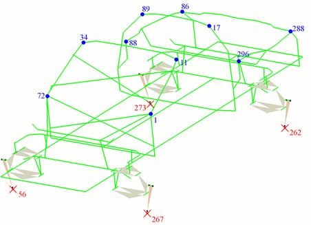
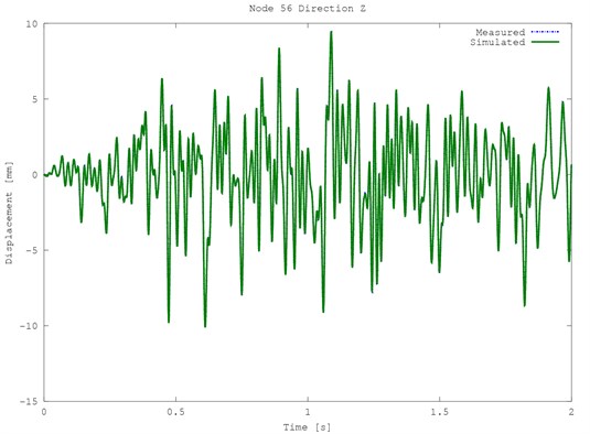
Fig. 2Exemplary time displacements of the structure for node 56, green line – simulated plot, blue dotted line – measured plot

3. Computer simulation

Model of the structure is presented in Fig. 1. It is mainly based on beam elements, but there are also applied mass, spring and damping elements. The model was kinematically excited along vertical direction in four nodes 56, 262, 267 and 273. The responses were registered along three directions in ten nodes 1, 11, 17, 34, 72, 86, 88, 89, 288 and 296. Time modal history was synthesized with the use of the twelve first modes for the period of time 2 s and step of integration 0.001 s.

All twelve modal displacements were identified with the use of Eq. (11). Then the generalized coordinates of the subsystem with the known motion ${\mathbf{q}}_g\left(t\right)$ were computed with the use of Eq. (14). Results for the selected node 56 are presented in Fig. 2. The obtained signals are nearly identical with the given one.

4. Conclusions

The results of computer simulation (virtual prototyping) showed very good compliance of the given signals of kinematic excitation with the computed ones. The latter also concerns conformity of the desired and simulated vibrations of the car body. It is possible to effectively compute kinematic excitations’ functions, even if the simulated and given signals are not the same. Numerical computations are effective due to the use of modal model of the car body. In case of real structures, modal model can be easily obtained with the use of experimental modal analysis techniques. Thus, the modal model parameters obtained during real experiments, can be applied for a purpose of virtual prototyping.

It should be noted that despite ability of good adjustment of the kinematic excitation function to real working conditions of the structure, virtual prototyping would not give an answer to the question what the fatigue endurance is. In order to determine fatigue endurance, suitable programme of experiments should be performed on the laboratory stand (number of cycles in a range of 10⁹), at kinematic excitation determined on a stage of virtual prototyping.

The economic criterion is fulfilled in the end. Laboratory investigations are cheaper than testing of ready transportation means during their routine operation.

References

-
Kaliński K. J., Buchholz C. Mechatronic design of strongly nonlinear systems on a basis of three wheeled mobile platform. Mechanical Systems and Signal Processing, 2014, http://dx.doi.org/10.1016/j.ymssp.2014.06.016.
Kruszewski J., Gawroński W., Wittbrodt E., Najbar F., Grabowski S. The Rigid Finite Element Method. Arkady, Warszawa, 1975, (in Polish).
Maia N. M. M., Silva J. M. M. Theoretical and Experimental Modal Analysis. Research Studies Press, Taunton, Somerset, England, 1997.
Heylen W., Lammens S., Sas P. Modal Analysis Theory and Testing. KU Leuven, Leuven, 2007.
Kaliński K. J. A Surveillance of Dynamic Processes in Mechanical Systems. Publishing House of Gdańsk University of Technology, Gdańsk, 2012, (in Polish).
About this article
The authors kindly acknowledge firms vMACH Engineering GmbH of Markt Indersdorf, Germany, and Macross GmbH of Munich, Germany, for providing the research with some experimental data concerned modal model of the car body, as well as – real kinematic excitations of chassis vehicles.