Abstract
Vibration signals of defective gears are usually non-stationary and masked by noise. As a result, the feature extraction of gear fault data is always an intractable problem, especially for multi-fault couple system (two or more fault types simultaneously occur in mechanical systems). Recently, an interesting crossover characteristic of nonlinear data is used to diagnose the different severities of gear faults. Nonetheless, it lacks of self-adaptivity. Consequently, a novel method for self-adaptive feature extraction using scaling crossover characteristics of signals and combining with least square support vector machine (LS-SVM) for multi-fault diagnosis of gearbox is proposed. Firstly, detrended fluctuation analysis (DFA) is introduced to analyze fractal properties and multi-scaling behaviors of vibration signal from multi-fault gearbox. The scale exponents are abrupt changed with the gradual increasing of time scales, which can be observed in the scaling-law curve. Secondly, a criterion based on a Quasi-Monte Carlo algorithm is developed to uncover optimal scaling intervals of scaling-law curve. Several different scaling regions are objectively measured in each of which a single scale exponent can be estimated. Thirdly, a three-dimensional vector, containing three scale exponents which carry definite physical meaning, is used as the feature parameter to describe the underlying dynamic mechanism hidden in gearbox vibration data. Lastly, these vectors are classified by LS-SVM. Moreover, the method of statistical parameters is exploited to classify the multi-fault vibration data which have been investigated by proposed method. The results show that the proposed method is sensitive to multi-fault vibration data of gearbox with similar fault patterns and has a better performance than other methods.
1. Introduction
As a key component of rotating machinery, gears are mostly subjected to progressive deterioration due to severe working conditions [1]. The condition of a gear directly affects the normal running of the machine or even the entire system. The faults caused by gear failures account for 10 % of the malfunctions in rotating machines and 80 % in the transmission machinery, respectively. Therefore, it is necessary and critical that the detection and diagnosis of gear faults are performed to prevent breakdown accidents and to minimize production loss.
Gearbox fault diagnosis has received intensive study for several decades and yet a few lectures focus on multi-fault diagnosis of gearbox. For example, wind turbine gearboxes have multi-gearing and multi-bearing [2]. It is usually difficult to diagnose their potential faults. Especially when multi-faults coexist, vibrations excited by several faults are combined with each other non-linearity and non-stationary. Among the available diagnosis techniques, vibration analysis is the most commonly used and efficient method. However, it is easily influenced by vibration sources from many cases, such as the meshing gears, shafts, and bearings. As a result, the vibration signals are usually quite complex and their analyses are interfered. So far many developed fault detection techniques focus on the evolution of statistical parameters (such as standard deviation, skew and kurtosis, etc.) as a function of time [3], or on frequency analysis [4]. More recently, a series of hybrid time-frequency techniques have been developed, such as wavelet, Wigner-Ville or correlated transforms [5-10]. Both frequency and hybrid techniques rely on the identification of the existing fault frequency. However, when used to analyze the complex gearbox vibration data, the previous methods often produce unsatisfactory results because of their respective drawbacks [11-13] especially to multi-fault gears which have many same feature frequencies. Therefore, the further researches on these methods are in progress, particularly for multi-fault diagnosis.
Recently, De Moura et al. [14, 15] firstly made a constructive attempt to apply DFA to gear and bearing fault diagnosis. In paper [14], DFA was used as a transform tool to compress gearbox vibration data containing 2048 points into the scaling-law curve of 37 values. The extracted the scaling-law curve, by which the relation between the fluctuation function and the time scale can be illustrated graphically in a log-log plot, fully expressed various working conditions contained in the original gearbox data. Afterwards, in paper [15], bearing vibration data containing 4096 points were transformed into the scaling-law curve of 37 values and the extracted the scaling-law curve wholly represented various conditions of severity defects in the original bearing data. Eventually, DFA method was proved to be an excellent tool for data compression. However, only a mono-fractal characteristic was used in [14] and [15], so that it was barely able to expose the underlying nonlinear dynamical mechanism hidden in multi-fractal time series. Lin et al. [16, 17] used DFA to analyze the scaling behavior of gearbox vibration data by a two-dimensional vector containing two scale exponents which carried definite physical meaning and could be used as feature parameters to describe the gearbox vibration data. It showed that DFA method was a powerful tool for uncovering the nonlinear dynamical characteristics buried in non-stationary time series and could capture minor changes of complex system conditions. However, the detections of crossover points and scale regions were relatively subjective since it has been made without rigorous statistical procedures and has generally been determined by eye balling or subjective observation. Crossover points and scale regions determined liked these may be spurious and problematic. It may not reflect the genuine underlying scaling behaviors of a time series.
Multi-scaling behaviors are often found in nature [18]. The identification of these characteristic scales is relevant for a complete understanding of the underlying multi-scale dynamics [19]. As stated by Shao et al. [20]: “there is no consensus on an objective determination approach of the scaling range, which plays a crucial role in the estimation of the scaling exponents”. If it has no solid theoretical foundations for the quantitative detection of the crossover time scales, it will produce a subtle issue when dealing with series which have more than one scaling behavior. The detections of crossover points and scale regions have been mainly done by the visualization of the log-log plot and the presence of seemingly different exponent values would be shown in the results [18]. Therefore, it is necessary to develop an independent criterion to estimate the optimal fitting regions of scaling-law curve. Crossover phenomena, i.e. the presence of crossover scales separating regimes with different scaling exponents, may be efficiently unveiled by applying regression analysis and statistical inference. One possibility is to study the local exponents by means of the log derivative plot and look for constant value regions, as suggested by Govindan et al. [21], Bashan et al. [22] and Lopez et al. [23]. However, the method only searched a single crossover point, making it difficult to apply in the cases of multi-crossover points. Additionally, Michalski [24] identified the optimal minimal and maximal scale sizes for persistent processes through a number of extensive Monte Carlo simulations. Moreover, Grech et al. [25] studied the relations between the scale region of artificial correlated and uncorrelated series and series length, Hurst exponent and goodness of fluctuation function linear fit in a given confidence level. Unfortunately, these methods needed to consume much time. In follows, a related approach using linear fit as a way to locate optimal scaling regions was proposed in paper [26]. This criterion based on goodness of linear fit might be naturally extended to other techniques requiring linear fits. It was not computationally prohibitive since it deals with relatively few points. The method will be developed and used in our study for the multi-fault diagnosis. The criterion grounded on a solid statistical foundation can describe multi-scaling behaviors of fractals. Through the regression analysis and statistical inference, we can identify the crossover time scales that cannot be detected by eye-balling observation and determine the number and locations of the genuine crossover points.
To evaluate the performance of the feature parameters characterizing the multi-fault gearbox, LS-SVM is suitably employed to differentiate the different fault types of gearbox. LS-SVM is an evolution of SVM. The simplicity and inherited advantages over SVM, such as excellent generalization ability and a unique solution, promote the applications of LS-SVM. The most important difference between them is that the loss function of LS-SVM is least square linear system rather than quadratic optimization. LS-SVM has been widely used as classifiers in machine fault diagnosis [27, 28]. LS-SVM will be regarded as classifiers in our study.
The paper is organized as follows. In Section 2, the DFA method is briefly described. Besides, the determinate criterion and identification method of crossover scales are presented. Then, the fame of gearbox multi-fault diagnosis is proposed. Section 3 provides the introduction for all types of vibration signals from multi-fault gearbox. The achieved results of proposed method compared with the analysis results of statistical parameters are investigated in Section 4. An in-depth discussion about the proposed method is given in Section 5. Conclusions of the proposed novel method for multi-fault diagnosis are drawn in the final section.
2. Theoretical backgrounds
2.1. Describe detrended fluctuation analysis (DFA)
Since the seminal study on DFA was proposed by Peng et al. [29], this technique has been widely used in time series analysis. The DFA aims to improve the evaluation of correlations in a time series by eliminating trends in the data. The method is described as follows.
1) Consider a signal , where , and is the length of the signal. An integrated time series of is obtained as:
where is the mean of given as:
2) Split series into non-overlapping windows with data points. denotes the round numbers. If is not divisible by , there are some remaining values at the end of the series . To solve this problem, the other segments are acquired but starting from . In this way, windows of data points are obtained.
3) Let be the index of the window. For each one of these windows it takes the polynomial of degree to fit the data in the window where is the data index. Then the local variance is obtained as Eq. (3). If is divided by, it simply repeats the values of :
where , must be the same for every step of this technique, determining the detrend polynomial order of analysis.
The averaged root mean square value, i.e. fluctuation function for the entire time series is given as:
4) Repeated all the above steps 1-3 for several values of in order to construct the relation between fluctuation function and time scale . The relation is presented in the form as:
By a double logarithmic operation, the parameter which is called the Hurst exponent or scale exponent can be evaluated. Simultaneously the relation between the fluctuation function and the time scale can be illustrated graphically by the scaling-law curve in a log-log plot. The value of indicates that there are no correlations or only short-term correlations [17]. If , the data are long-term correlated. With the increasing of the persistent long-range correlation of data is enhanced. The case of corresponds to long-term anti-correlations, meaning that large fluctuation is more possible to be followed by small values.
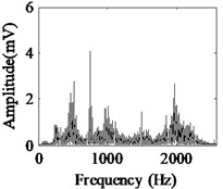
In fact, the complex fractal time series generally do not exhibit mono-scaling behavior characterized by a single scaling exponent. Multi-scaling behaviors are actually very common in natural phenomena. An example for vibration signal of multi-fault gearbox and its scaling-law curve analyzed by DFA is shown in Fig. 1. There are two obvious crossover points which are shown as the square points described in Fig. 1(b). As a result, the two crossover points can be employed to divide the whole scaling-law curve into three different scale regions, in each of which a single scale exponent can be estimated. However, it hardly determines the scale exponent without a theoretical model for multi-scaling behaviors. If the determinations of these regions are subjective, the results derived from different analysis of the same series can not be consistent. Therefore, an independent criterion to estimate the optimal scale region of scaling-law curve is developed in the Subsection 2.2.
Fig. 1Example for the vibration data of muti-fault gearbox with multi-scaling behaviors
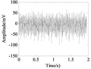
a) Time domain signal
b) Scaling-law curve obtained by DFA
2.2. The method of uncovering optimal scale intervals
The optimal scale regions of time series with crossover characteristics can be objectively and efficiently estimated by using the method of Quasi-Monte Carlo. The Quasi-Monte Carlo method is described as follows.
1) Suppose that is a time series which has given scales where the fluctuation function , is calculated.
2) Define a number of data points. In practice, the parameter must be less than the length of minimum scale region. A detailed discussion with the selection of parameter is given at the end of this subsection.
3) Calculate the logarithmic series and , .
4) Define a matrix of default values equal to 0.
5) Compute all non-zero elements of according as:
where is the coefficient of determination with the linear fit of versus between the logarithmic time scale and , and .
6) Sort all non-zero values in decreasing order while keeping a record of their original subindices. The first element of this list will then provide the first optimal fitting scale interval. If there are repeated values in , sorting requires an extra criterion that the longest interval length is selected. The slope of linear fit is regard as scale exponent of the scale interval.
7) Eliminate searched interval in step 6. Then, repeat above steps 2 to 6. The next optimal region can be searched in remaining interval until all linear regions are uncovered.
This algorithm is called as Quasi-Monte Carlo since it actually performs all possible fits at least data points between scales and . In order to more clearly clarify how to operate the method for multi-fault vibration signals, there are two projects used to illustrate the operational process subsequently.
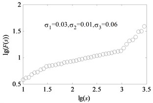
A simple artificial series is performed by this method. The 126 equally spaced points are generated in interval of [1, 3.5]. Then, the Eq. (7) is calculated.
where , , are generated as a set of uniform random numbers of variances , , used as the additive noise. Then the artificial fluctuation functions and scales are generated with series and according to:
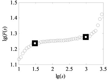
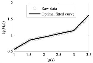
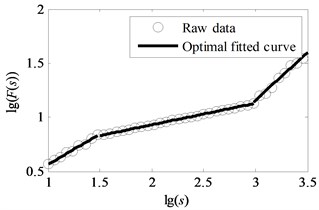
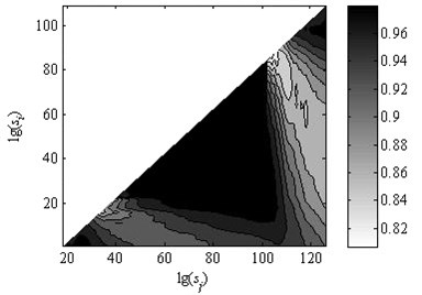
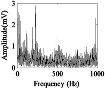
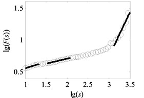
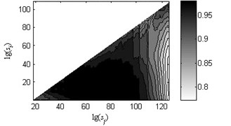
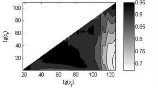
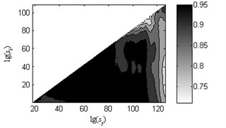
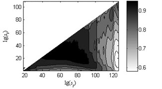
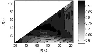
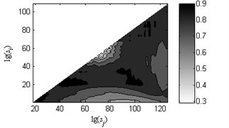
Consider two kinds of situations. One is that the relationship of variances for random numbers , , , is and the other one is . The data points are set as 18. The analysis results of artificial series by the method of uncovering optimal fitting scale intervals are shown in Fig. 2 and Fig. 3 respectively. It can be seen that that the fitted curves are perfectly coincident with original data depicted in Fig. 2(b) and Fig. 3(b). The slopes of two examples are (0.5464, 0.2021, 0.9377) and (0.2002, 0.5505, 0.9228) which approximate to the genuine value (0.55, 0.20, 0.90). Moreover, the order of the obtained linear region is in accordance with the sizes of , , . As seen in Fig. 2(c) and Fig. 3(c), the coefficients of determination approach to one. It demonstrates that the method of uncovering optimal scale intervals is reliable.
It should be remarked that the key of the method for uncovering optimal scale intervals is to set up the parameter . As mentioned in paper [26], the computing time for this implementation might be approximated by:
where is constant. is the number of active cores. This inverse proportionality is due to the fact that elements in the matrix are independent of each other, therefore enabling the possibility to split the processing task.
Fig. 2Analysis results of series with noise

a) Series with noise
b) Fitting result by the method of uncovering optimal fitting scale intervals
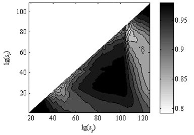
c) Coefficient of determination of the linear fit
Fig. 3Analysis result of series with noise
a) Series with noise
b) Fitting result by the method of uncovering optimal fitting scale intervals
c) Coefficient of determination of the linear fit
According to Eq. (9), the large parameter is conducive to reducing computing time. Moreover, the reasonable large parameter makes more obvious statistical sense for the linear fit. However, the parameter should be less than the data points of the shortest scale regions. Because the parameter is too large it could cause a poor statistical sense. As delineated in Eq. (7), the data points of the scale region are 42. Therefore, the data points are set as 18 which is a tradeoff between computing time and statistical sense.
2.3. The method of LS-SVM
As an improvement of Vapnik’s standard SVM [30], LS-SVM classifier [31] leads to solve a linear system instead of a quadratic optimization method. Its objective function is formulated as:
where stands for the th desired output. denotes a nonlinear mapping of the th input sample of the training data set from the primal space to the feature space. is viewed as a form of a “regularization” parameter which controls the tradeoff between the complexity of the machine and the number of non-separable points. is a vector which determines the orientation of a separating hyperplane. is the slack variables.
In general, may potentially become infinite dimensional so that a separating hyper-plane does not exist. Hence the constrain is relaxed by introducing slack variables The corresponding Lagrangian equation is built as:
where () is the Lagrange multiplier.
Then support vectors are got by Karush-Kuhn-Tucker (KKT) condition. The classifier in the dual space takes the form as Eq. (12). The detailed procedure can consult in paper [32]:
where is called the kernel function that must satisfy Mercer condition.
2.4. Frame of the novel method for feature extraction using crossover characteristics
As a result, the method of uncovering optimal fitting scale intervals can be employed to divide the whole scaling-law curve into several different scaling regions, in each of which a single scale exponent can be estimated. Taking advantage of the natural crossover characteristics of the scaling-law curve, a novel method for self-adaptive feature extraction using crossover characteristics is proposed in this study. The whole procedure of the proposed novel method can be decomposed as the following four steps:
1) Analyze the vibration signal of multi-fault gearbox by DFA and obtain the scaling-law curve described in Subsection 2.1.
2) Segment the entire scaling-law curve into several different scaling regions by the method of uncovering optimal scale intervals demonstrated in Subsection 2.2.
3) Extract the scale exponents in each scale region as the feature parameters and utilize them to characterize the fault types.
4) Use the method of LS-SVM to classify the feature parameters obtained in the third step.
3. Capture vibration signals of multi-fault gearbox
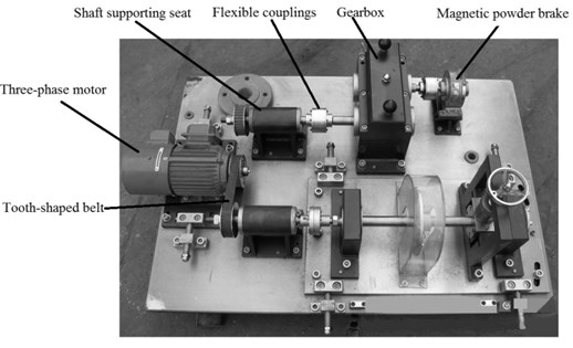
Gear failures including the localized faults (pit, broken) and distributed fault (worn), as well as coupled fault in power train perhaps cause catastrophic accidents. Therefore, an early recognition of the gear faults is critical for normal operation of a gearbox [33]. Our paper focuses on investigating the multi-fault gearbox. As illustrated in Fig. 4, all trials are performed on a specially designed bench which is composed of a one phase input and three-phase output motor (with nominal power of 0.75 kW and nominal rotation frequency of 1500 rpm), the shaft supporting seats, a flexible coupling, a gearbox and a magnetic powder brake. The rotation of motor is controlled by a frequency inverter. The maximum braking torque of magnetic powder brake is 5 N⋅m. The gearbox contains two gears (pinion and wheel gear). The gear parameters are displayed in Table 1.
Fig. 4Bench of multi-fault gearbox
There are six fault types of gearbox: normal, a single broken tooth of wheel, a single pit of wheel, a single worn of pinion, coupled fault of wheel pit and pinion worn, coupled fault of wheel broken and pinion worn which are considered in this experimental case. For brevity, the six typical fault types of gearbox are named as Type-1, Type-2, Type-3, Type-4, Type-5 and Type-6 respectively. Two kinds of rotating conditions (880 rpm and 1500 rpm) are employed for these six fault types of gearbox. When the rotational speed of the motor is 880 rpm, there are four kinds of loads which are the absence of external load and loads of three different currents of magnetic powder brake respectively. Hereby, load-1, load-2 and load-3 represent 0.2 ampere (A), 0.1 A and 0.05 A current of magnetic powder brake, respectively. When the rotational speed is 1500 rpm, a unique absence of external load is set up for all fault types of gearbox. Therefore, each fault type of gear contains five running conditions. 44 data samples are collected for each working condition of one fault type in this experiment. So a total of 1320 data samples are obtained on the designed bench. The sensor used is a piezoelectric accelerometer (DH131E) mounted on the flat surface of gearbox. The sampling frequency is 5120 Hz for all conditions. Each data sample is composed of 10000 data points.
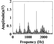
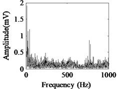
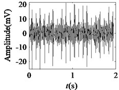
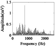
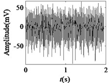
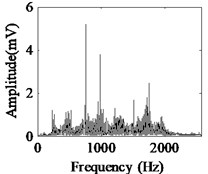
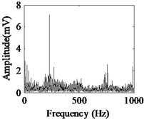
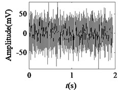
A group of vibration signals for six fault types of gearbox under load-1 with rotational speed of 880 rpm are expressed in Fig. 5.
Table 1Gear parameters
Gear | Teeth | Module (mm) | Pressure angle (deg.) | Materials |
Pinion | 55 | 2 | 20 | S45C |
Wheel | 75 | 2 | 20 | S45C |
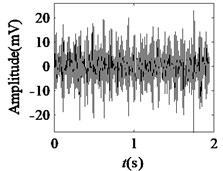
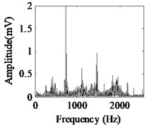
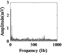
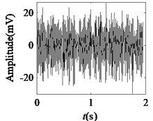
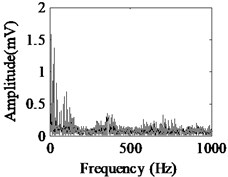
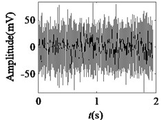
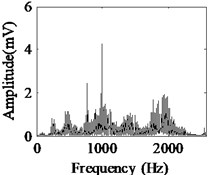
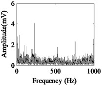
Fig. 5Acquired raw data, FFT spectrum and envelope spectrum under load-1 with rotational speed of 880 rpm: a), b), c) Type-1; d), e), f) Type-2; g), h), i) Type-3; j), k), l) Type-4; m), n), o) Type-5; p), q), r) Type-6
a)
b)
c)
d)
e)
f)
g)
h)
i)
j)
k)
l)
m)
n)
o)
p)
q)
r)
It can be seen from the first column of Fig. 5 that the raw vibration signals of all fault types of gearbox are heavily contaminated by noise. In general, the feature component of periodic impulse is often encountered when faults occur on gear teeth. However, this characteristic is not obvious in the time waveforms of the raw data except the pit of wheel shown in Fig. 5(g). In addition, the Fast Fourier Transform (FFT) spectral for gear faults should be marked by both the rotational frequency and gear meshing frequency as well as their harmonic based on the study of mechanism of gear faults [34]. As demonstrated in the second column of Fig. 5, this phenomenon cannot be observed well in FFT spectra of all fault types of gearbox. Moreover, the vibration signals for the different fault types of gearbox have almost the same representation in frequency domain. Similarly, the distinct features cannot be obtained from the envelope spectra of all fault types described in the third column of Fig. 5, even if Type-1 can be differentiated from the other types. As a result, it is infeasible and unreliable to recognize the gear states through the waveforms of FFT spectrum and envelope spectrum. Therefore, the proposed method described in Subsection 2.4 is used to diagnose the multi-fault gearbox in Section 4.
4. Experiment results for multi-fault diagnosis based on the proposed novel method
This section is made of two subsections. According to scaling crossover characteristics of multi-fault data, the feature parameters obtained from optimal fitting scale intervals are displayed in Subsection 4.1. The performances of the proposed novel method for the multi-fault diagnosis of gearbox are evaluated in Subsection 4.2. Furthermore, compared with the proposed method, some statistical parameters (pulse factor, kurtosis and form factor) in the time domain and the combination of scale exponents and statistical parameters are also explored to characterize the multi-fault data in Subsection 4.2.
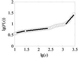
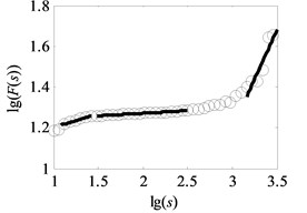
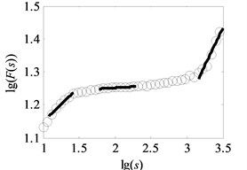
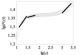
Fig. 6Analysis result of uncovering optimal scale intervals under load-1 with rotational speed 880 rpm
a) Type-1
b) Type-2
c) Type-3
d) Type-4
e) Type-5
f) Type-6
4.1. Extract the feature parameters from optimal fitting scale intervals
The vital step of the proposed method is the extraction of feature parameters. In this subsection, the method of uncovering optimal scale intervals in Subsection 2.2 is used to analyze the vibration data of multi-fault gearbox. As suggested in paper [16], the degree of DFA introduced in Subsection 2.1 which can be obtained by attempting different orders is finally set as one. Additionally, the range for data points of non-overlapping windows is from 10 to 3000, i.e. the interval of logarithmic () is set to range from 1 to 3, described in paper [17]. In our study, under the same assumptions, the degree of DFA is 1 and the range for the data points of non-overlapping windows is from 10 to 3162, i.e. the interval of is uniformly set to range from 1 to 3.5 with the spacing of 0.02 to observe the analysis results in the larger windows. As depicted in Fig. 1(b) and Fig. 6(a)-(f), the scaling-law curves obtained by DFA for all fault types of gearbox clearly exhibit two crossover points. The scaling-law curves can be roughly divided into three scaling regions by using these crossover points where the -coordinates of two crossover points are close to and respectively. Therefore, the ranges of three scale regions approximate to , , and respectively. As displayed in Fig. 6(a)-(f), the first and third linear regions have a shorter length than the second region. The shortest length of these linear intervals approximates to 25. To uncovering the optimal scale intervals, the data points are set as 18 which is a tradeoff between computing time and statistical sense as explained in Subsection 2.2.
Fig. 7Coefficients of determination (R2) of the linear fitting under load-1 with rotational speed 880 rpm
a) Type 1
b) Type 2
c) Type 3
d) Type 4
e) Type 5
f) Type 6
As shown in Fig. 6, the black heavy lines represent the optimal scale intervals fitted by the criterion based on a Quasi-Monte Carlo algorithm. Fig. 6(a)-(f) manifest that the optimal fitted lines can completely depict the outline of scaling-law curves. It can be seen from Fig. 7(a)-(f) that the coefficients of determination before the non-overlapping window of are more apparent than the remaining parts. That is, the linearity of first and second linear regions , has a better performance than the one of the third region . As a consequence, the order of the obtained linear regions may be , and or , and which are consistent with analysis in Subsection 2.2. Lastly, three scale exponents, in turn, are estimated from these linear regions by least square fitting. Afterwards three scale exponents are determined, the sequence of scale exponents should be rearranged to conform the original order , and for uniformly forming a standard vector employed in Subsection 4.2 as the input samples. Table 2 reports the three scale exponents for six fault types of gearbox under load-1 with rotational speed of 880 rpm. As reported in Table 2, the scale exponents in the first two scaling regions are less than 0.5 and hence the corresponding data exhibit extremely strong anti-persistent long-range correlations while the opposite situation is shown in third linear region. In next subsectioon, we will present the discriminability of the features vector which is expressed as:
where , and mean the three scale exponents in sequence.
Table 2Three scale exponents for six fault types of gearbox under load-1 with speed of 880 rpm
Fault type | SE1 | SE2 | SE3 | Fault type | SE1 | SE2 | SE3 |
Type 1 | 0.1798 | 0.1938 | 1.6275 | Type 4 | 0.1189 | 0.0187 | 1.3390 |
Type 2 | 0.2319 | 0.0707 | 1.6368 | Type 5 | 0.2107 | 0.0141 | 0.4584 |
Type 3 | 0.2413 | 0.1327 | 1.2454 | Type 6 | 0.1717 | 0.0364 | 0.1584 |
4.2. Compare the classified peformance of proposed method with statistical parameters
In general, it is difficult to identify fault types by directly observing features. In this section, LS-SVM are used to realize the recognition for multi-fault gearbox.
As described in Subsection 2.3, the primary principle of LS-SVM which is an intelligent learning algorithm and derived from the work of Vapnik et al. [30, 35] is to map the input from the primal space to the feature space by kernel function shown in Eq. (12). The selection of kernel function will affect the learning ability and generalization of LS-SVM. Since the Gaussian Radial Basis Function (RBF) kernel always have a superior performance than the other kinds of kernel functions in many practical applications [36], the RBF kernel which is shown in Eq. (13) is adopted in our research. As well, the RBF kernel is a better choice than other kernels like polynomial kernel because it has lesser hyper-parameters and so the problem becomes less computationally intensive. In addition, the LS-SVM is designed intrinsically for binary classification which is not suitable for multi-class of multi-fault diagnosis. However, in our paper, a six-class classification problem should be implemented by extending the binary classification. Many approaches have been considered for multi-class classification issue, such as “one-against-one”, “one-against-all”, and directed acyclic graph SVM [37]. “one-against-one” is to break down the multi-class problem into a number of smaller binary problems. “one-against-all” considers all classes at once and solves the multi-class problem in one step. In general, “one-against-all” is computationally more expensive to solve a multi-class problem than “one-against-one”. Hsu and Lin [38] discussed the characteristics of these methods and pointed out that the “one-against-one” method is more suitable for practical application than other methods. In this study, we select the “one-against-one” to identify the different fault types:
where is the bandwidth of the Gaussian RBF kernel function which controls the degree of non-linearity of the model.
In order to make fair and objective evaluation for each type of multi-fault gearbox, two key parameters in LS-SVM, and , which play an important role in the classification performance for LS-SVM are optimized by grid searching [39]. The search scopes of parameters and are between 0 and 2 with spacing of 0.1. As mentioned in Section 3, 44 data samples for each operating condition of one fault type are collected from the surface of gearbox. 44 samples are divided into training samples and testing samples, respectively. 15 samples are selected as training samples and the remaining 29 samples are regarded as testing samples. Therefore, a total number of training samples are 90 and testing samples are 174 for six fault types of gearbox under one working condition. The objective function of grid searching method is the average percentage of correct classification, i.e. the ratio of the total number of training samples correctly classified to the total number of training samples.
As displayed in Fig. 8, five of the training samples of are misclassified, yielding the maximum average percentage of classification accuracy (CA) which is calculated as Eq. (15) is 94.4 % under load-1 with rotational speed of 880 rpm when and are equal to 1.1 and 1.6 respectively:
Fig. 8Optimal training results are obtained by grid searching in LS-SVM
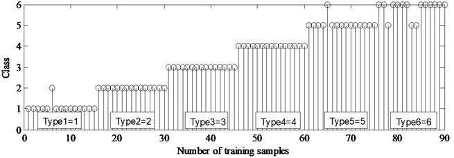
Fig. 9Classification results in testing samples by LS-SVM
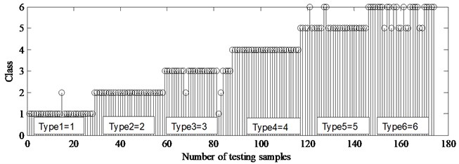
To illustrate the process concretely, the classification results of in testing phases are drawn in Fig. 9. It can be seen from Fig. 9 that 16 of the testing samples are misclassified, yielding the success rates 90.8 %. Among them, 2 samples of type-1, 3 samples of type-3, 3 samples of type-5 and 8 samples of type-6 are misclassified respectively. For brevity, the CA of testing samples obtained by the proposed method for all types of multi-fault data are listed in Tables 3-4.
Additionally, compared with the proposed method, the vector of statistical parameters expressed as Eq. (16) is employed to examine the same multi-fault data which have been investigated by proposed method:
where , and denote pulse factor, kurtosis and form factor, respectively.
The main parameters in LS-SVM are set in the same way as ones in our proposed method. The analysis results of testing samples about vector are demonstrated in Table 5 and Table 6.
As illustrated in Table 3 and Table 5, the classified performances of our proposed method are obviously over the performances of statistical parameters in all fault types of gearbox except the slightly less CA for the load-1 of type-5 and load-2 of type-6. Similarly, the comparisons of Table 4 and Table 6 clearly indicate that the performances of proposed method are also over the performances of statistical parameters at the absence of external load. Especially, zero correct classification crops up at type-4 and type-6 of 880 rpm shown in Table 6. As observed in Table 3, the classified performance of heavy load (load-1) is better than light load (load-2). Table 4 presents that the working condition with highly rotational speed has a slightly helpful for improving CA. The contrasts of Table 3 and Table 4 imply that the performances of the absence of external load are slightly poor. The classified results of statistical parameters are unstable and lowly accurate depicted in Table 6.
Table 3Classification accuracy (CA) of testing samples under load-1, -2, -3 with 880 rpm by proposed method
Fault type | Load-1 (CA %) | Load-2 (CA %) | Load-3 (CA %) | Fault type | Load-1 (CA %) | Load-2 (CA %) | Load-3 (CA %) |
Type 1 | 93.10 | 86.21 | 100.00 | Type 4 | 100.00 | 100.00 | 96.55 |
Type 2 | 100.00 | 96.55 | 82.76 | Type 5 | 89.66 | 79.31 | 100.00 |
Type 3 | 89.66 | 79.31 | 72.41 | Type 6 | 72.41 | 65.52 | 86.21 |
Table 4Classification accuracy (CA) of testing samples under unload with rotational speed of 880 and 1470 rpm respectively by proposed method
Fault type | 880 rpm unload (CA %) | 1470 rpm unload (CA %) | Fault type | 880 rpm unload (CA %) | 1470 rpm unload (CA %) |
Type 1 | 86.21 | 89.66 | Type 4 | 93.10 | 100.00 |
Type 2 | 82.76 | 96.55 | Type 5 | 96.55 | 55.17 |
Type 3 | 72.41 | 86.21 | Type 6 | 68.96 | 72.41 |
Table 5Classification accuracy (CA) of testing samples in statistical features (pulse factor, kurtosis and form factor) under load-1, -2, -3 with 880 rpm
Fault type | Load-1 (CA %) | Load-2 (CA %) | Load-3 (CA %) | Fault type | Load-1 (CA %) | Load-2 (CA %) | Load-3 (CA %) |
Type 1 | 86.21 | 58.62 | 100.00 | Type 4 | 58.62 | 96.55 | 58.62 |
Type 2 | 37.93 | 62.07 | 79.31 | Type 5 | 100.00 | 72.41 | 68.96 |
Type 3 | 44.83 | 62.07 | 72.41 | Type 6 | 44.83 | 100.00 | 55.17 |
Table 6Classification accuracy (CA) of testing samples in statistical features under absence of external load with rotational speed of 880 and 1470 rpm respectively
Fault type | 880 rpm unload (CA %) | 1470 rpm unload (CA %) | Fault type | 880 rpm unload (CA %) | 1470 rpm unload (CA %) |
Type 1 | 100.00 | 44.83 | Type 4 | 0 | 62.07 |
Type 2 | 86.21 | 13.79 | Type 5 | 100.00 | 48.28 |
Type 3 | 20.69 | 89.66 | Type 6 | 0 | 13.79 |
Successively, to further improve the classified performance of proposed method, one idea that vector which is form as Eq. (17) (the combination of three scale exponents and three statistical parameters ) is attempted to used to characterize the types of multi-fault gearbox:
where represent the combination of vector and vector .
The main parameters in LS-SVM are set in the same way as ones in the proposed method. The classified performances of vector are presented in Table 7 and Table 8. From the comparison of Table 3 and Table 7, the combination of these parameters has a better performance than the single vector . Identically, Table 4 and Table 8 state that the performances of novel idea are superior to the single vector under working condition of the absence external load. As reported in Table 7, it must be point out that the CA is 100 % for all fault types under load-1 with rotational speed of 880 rpm.
Table 7Classified performances of the combination of scale exponents and time domain features at condition of load-1, -2, -3 with 880 rpm
Fault type | Load-1 (CA %) | Load-2 (CA %) | Load-3 (CA %) | Fault type | Load-1 (CA %) | Load-2 (CA %) | Load-3 (CA %) |
Type 1 | 100.00 | 100.00 | 100.00 | Type 4 | 100.00 | 100.00 | 93.10 |
Type 2 | 100.00 | 93.10 | 100.00 | Type 5 | 100.00 | 100.00 | 86.21 |
Type 3 | 100.00 | 86.21 | 96.55 | Type 6 | 100.00 | 100.00 | 100.00 |
Table 8Classified performances of the combination of scale exponents and time domain features at condition of 880, 1470 rpm and unload
Fault type | 880 rpm unload (CA %) | 1470 rpm unload (CA %) | Fault type | 880 rpm unload (CA %) | 1470 rpm unload (CA %) |
Type 1 | 93.10 | 96.55 | Type 4 | 86.21 | 100.00 |
Type 2 | 96.55 | 96.55 | Type 5 | 100.00 | 62.07 |
Type 3 | 86.21 | 89.66 | Type 6 | 72.41 | 68.96 |
5. Discussions
In this paper, the crossover characteristics of the scaling-law curve was introduced to explore complex multi-fault data and a novel method for multi-fault diagnosis of gearbox was proposed based on DFA, a Quasi-Monte Carlo algorithm and LS-SVM. Applied to multi-fault diagnosis of realistic gearbox, the proposed method in this paper can produce satisfactory performances in distinguishing different fault types of gearbox. Moreover, compared with statistical parameters, the combination of DFA and a Quasi-Monte Carlo algorithm perform better in feature extraction of gearbox vibration data.
Despite being a powerful tool for detecting the different fault types of gearbox, DFA still encounters some problems including discontinuities between trends of two neighboring data segments and practical difficulties in determining the type of the fitting polynomial [20]. Therefore, considerable efforts to resolve the problems existing in the original DFA are still required. This work lies beyond the scope of this study and will be carried out in future. In addition, data points have an effect on extracting precision of scale exponents. As a consequence, too large data size may lead to a poor result, whereas too small size may cause an increase in time cost. In our paper, data points which are set as 18 are reasonable and yet may not be optimal. Therefore, another problem which requires some research in future is how to determine a more appropriate data size for the method of uncovering optimal scale intervals.
In general, the overall procedure for a fault diagnosis scheme can be stated in four steps: data acquisition, signal processing, feature extraction, feature reduction and diagnostics (classifiers). The critical step in this process is to extract reliable features which are representative of the condition of gearbox. In our study, the feature extraction is chosen as the key research and LS-SVM is only regarded as a tool for evaluating the performances of feature extraction. In fact, as reported in Table 3 and Table 7, CA of testing samples approximate to 90 % for all types of multi-fault gearbox when the searching scope of parameters and are limited between 0 and 2. It is proved that the proposed method of feature extraction is very effective. Certainly, it is without doubt that CA of testing samples can be further enhanced when the other optimization methods such as genetic algorithm and particle swarm optimization [27] are used to tune parameters and on a larger scale, which is a direction for further studies.
Furthermore, although the real multi-fault data collected from a laboratory test were explored in this paper, the proposed method which uncovers the underlying nonlinear dynamical mechanism hidden in time series from the view of data compression and multi-fractal could avoid the effect of noise in some extent and weaken the interference of non-stationary factors. Therefore, the fault diagnosis results in our study can provide good references for improving the layout of rotating machinery. Of course, modern rotating machinery such as wind turbine gearboxes has multi-gearing and multi-bearing. The dynamic responses of these components are complex and interfering with each other. When multi-fault of gears and bearing coexist in real world industrial situation, it makes the observed vibration signals rather complex, which makes it difficult to identify each fault. More research is needed to be done in the future.
6. Conclusions
1) A novel method of uncovering optimal scale intervals which can avoid the situations of spurious and problematic corssover points and scale regions and make the scale exponents self-adaptively extracted is proposed.
2) The classification results show that the proposed novel method is more effective than statistical parameters for multi-fault diagnosis. The load and rotational speed are the influenced factors of correct classification. The heavy load and high rotating speed are more conducive to increasing diagnostic reliability.
3) The combinations of scale exponents and statistical parameters further enhance the CA. The CA is up to 100 % under load-1 with rotational speed 880 rpm for all fault types. It is proved that the united idea could be further developed in multi-fault diagnosis of gearbox.
Furthermore, the multi-fault conditions with different fault types are more general situation in practice. Thus, it is of considerable practical significance to analyze these situations. Also, the proposed method can provide a reference for the fault diagnosis of other rotating machinery.
References
-
Fakhfakh T., Chaari F., Haddar M. Numerical and experimental analysis of a gear system with teeth defects. The International Journal of Advanced Manufacturing Technology, Vol. 25, Issue 5, 2005, p. 542-550.
-
Wang Z., Han Z., Gu F., et al. A novel procedure for diagnosing multiple faults in rotating machinery. ISA Transactions, 2014.
-
Li C. J., Limmer J. D. Model-based condition index for tracking gear wear and fatigue damage. Wear, Vol. 241, Issue 1, 2000, p. 26-32.
-
Randall R. B. A new method of modeling gear faults. Journal of Mechanical Design, Vol. 104, Issue 2, 1982, p. 259-267.
-
Wang W. J., McFadden P. D. Early detection of gear failure by vibration analysis I. Calculation of the time-frequency distribution. Mechanical Systems and Signal Processing, Vol. 7, Issue 3, 1993, p. 193-203.
-
Wang W. J., McFadden P. D. Early detection of gear failure by vibration analysis II. Interpretation of the time-frequency distribution using image-processing techniques. Mechanical Systems and Signal Processing, Vol. 7, Issue 3, 1993, p. 205-215.
-
Wang W. J., McFadden P. D. Application of wavelets to gearbox vibration signals for fault detection. Journal of Sound and Vibration, Vol. 192, Issue 5, 1996, p. 927-939.
-
Lin J., Zuo M. J. Gearbox fault diagnosis using adaptive wavelet filter. Mechanical Systems and Signal Processing, Vol. 17, Issue 6, 2003, p. 1259-1269.
-
Padovese L. R. Hybrid time-frequency methods for non-stationary mechanical signal analysis. Mechanical Systems and Signal Processing, Vol. 18, Issue 5, 2004, p. 1047-1064.
-
Fan X., Zuo M. J. Gearbox fault detection using Hilbert and wavelet packet transform. Mechanical Systems and Signal Processing, Vol. 20, Issue 4, 2006, p. 966-982.
-
Huang N. E., Shen Z., Long S. R., et al.The empirical mode decomposition and the Hilbert spectrum for nonlinear and non-stationary time series analysis. Proceedings of the Royal Society of London A: Mathematical, Physical and Engineering Sciences, Vol. 454, 1998, p. 903-995.
-
Wu Z., Huang N. E. Ensemble empirical mode decomposition: a noise-assisted data analysis method. Advances in Adaptive Data Analysis, Vol. 1, Issue 1, 2009, p. 1-41.
-
Frei M. G., Osorio I. Intrinsic time-scale decomposition: time-frequency-energy analysis and real-time filtering of non-stationary signals. Proceedings of the Royal Society A: Mathematical, Physical and Engineering Science, Vol. 463, Issue 2078, 2007, p. 321-342.
-
De Moura E. P., Vieira A. P., Irmão M. A. S., et al. Applications of detrended-fluctuation analysis to gearbox fault diagnosis. Mechanical Systems and Signal Processing, Vol. 23, Issue 3, 2009, p. 682-689.
-
De Moura E. P., Souto C. R., Silva A. A., et al. Evaluation of principal component analysis and neural network performance for bearing fault diagnosis from vibration signal processed by RS and DF analyses. Mechanical Systems and Signal Processing, Vol. 25, Issue 5, 2011, p. 1765-1772.
-
Lin J., Chen Q. Fault diagnosis of gearboxes based on the double-scaling-exponent characteristic of nonstationary time series. Chinese Journal of Mechanical Engineering, Vol. 48, Issue 13, 2012, p. 108-114.
-
Lin J., Chen Q. A novel method for feature extraction using crossover characteristics of nonlinear data and its application to fault diagnosis of rotary machinery. Mechanical Systems and Signal Processing, Vol. 48, Issue 1, 2014, p. 174-187.
-
Ge E., Leung Y. Detection of crossover time scales in multifractal detrended fluctuation analysis. Journal of Geographical Systems, Vol. 15, Issue 2, 2013, p. 115-147.
-
Du W., Tao J., Li Y., et al. Wavelet leaders multifractal features based fault diagnosis of rotating mechanism. Mechanical Systems and Signal Processing, Vol. 43, Issue 1, 2014, p. 57-75.
-
Shao Y. H., Gu G. F., Jiang Z. Q., et al. Comparing the performance of FA, DFA and DMA using different synthetic long-range correlated time series. Scientific Reports, 2012.
-
Govindan R. B., Wilson J. D., Preißl H., et al. Detrended fluctuation analysis of short datasets: an application to fetal cardiac data. Physica D: Nonlinear Phenomena, Vol. 226, Issue 1, 2007, p. 23-31.
-
Bashan A., Bartsch R., Kantelhardt J. W., et al. Comparison of detrending methods for fluctuation analysis. Physica A: Statistical Mechanics and its Applications, Vol. 387, Issue 21, 2008, p. 5080-5090.
-
López J. L., Contreras J. G. Performance of multifractal detrended fluctuation analysis on short time series. Physical Review E, Vol. 87, Issue 2, 2013, p. 1-9.
-
Michalski S. Blocks adjustment-reduction of bias and variance of detrended fluctuation analysis using Monte Carlo simulation. Physica A: Statistical Mechanics and its Applications, Vol. 387, Issue 1, 2008, p. 217-242.
-
Grech D., Mazur Z. On the scaling ranges of detrended fluctuation analysis for long-term memory correlated short series of data. Physica A: Statistical Mechanics and its Applications, Vol. 392, Issue 10, 2013, p. 2384-2397.
-
Gulich D., Zunino L. A criterion for the determination of optimal scaling ranges in DFA and MF-DFA. Physica A: Statistical Mechanics and its Applications, Vol. 397, Issue 1, 2014, p. 17-30.
-
Zheng H. B., Liao R. J., Grzybowski S., et al. Fault diagnosis of power transformers using multi-class least square support vector machines classifiers with particle swarm optimisation. Electric Power Applications, Vol. 5, Issue 9, 2011, p. 691-696.
-
Fernández F. D., Martínez R. D., Fontenla R. O., et al. Automatic bearing fault diagnosis based on one-class v-SVM. Computers & Industrial Engineering, Vol. 64, Issue 1, 2013, p. 357-365.
-
Peng C. K., Buldyrev S. V., Havlin S., et al. Mosaic organization of DNA nucleotides. Physical Review E, Vol. 49, Issue 2, 1994, p. 1685-1689.
-
Vapnik V. N. Statistical Learning Theory, John Wiley and Sons, New York, 1998.
-
Chang C. C., Lin C. J. Libsvm: A library for support vector machines. ACM Transactions on Intelligent Systems and Technology, Vol. 2, Issue 3, 2011, p. 1-27.
-
Widodo A., Yang B. S. Support vector machine in machine condition monitoring and fault diagnosis. Mechanical Systems and Signal Processing, Vol. 21, Issue 6, 2007, p. 2560-2574.
-
Baydar N., Ball A. A comparative study of acoustic and vibration signals in detection of gear failures using Wigner-Ville distributions. Mechanical Systems and Signal Processing, Vol. 15, Issue 6, 2001, p. 1091-1107.
-
Li Z., Yan X., Yuan C., et al. Virtual prototype and experimental research on gear multi-fault diagnosis using wavelet-autoregressive model and principal component analysis method. Mechanical Systems and Signal Processing, Vol. 25, Issue 7, 2011, p. 2589-2607.
-
Boser B. E., Guyon I. M., Vapnik V. N. A training algorithm for optimal margin classifiers. Proceedings of the Fifth Annual Workshop on Computational Learning Theory, 1992, p. 144-152.
-
Yang J., Zhang Y. Application research of support vector machines in condition trend prediction of mechanical equipment. Advances in Neural Networks, Vol. 3498, Issue 3, 2005, p. 857-864.
-
Cui J., Wang Y. A novel approach of analog circuit fault diagnosis using support vector machines classifier. Measurement, Vol. 44, Issue 1, 2011, p. 281-289.
-
Hsu C. W., Lin C. J. A comparison of methods for multiclass support vector machines. IEEE Transactions on Neural Networks, Vol. 13, Issue 2, 2002, p. 415-425.
-
Saidi L., Ali J. B., Fnaiech F. Application of higher order spectral features and support vector machines for bearing faults classification. ISA Transactions, 2014.
About this article

This research was supported by Aviation Science Foundation of China (Grant Number 2012ZD52054) and also supported by Science Combined Project of Nanjing University of Aeronautics and Astronautics (NZ2015103).
