Logistic analysis of economic cycles

1. Introduction

In the surrounding environment we witness a number of recurrent phenomena. These recurrences are related with the position of the elements, condition of the phenomenon and similar characteristics. In this paper we are going to investigate the fluctuations of the economic conditions, the potential and reasons of their recurrences.

At first glance it appears that economic development should be consistent. Yet, the practice indicates the opposite. When examining the consistent patterns of economic cycles, a number of scholars distinguish four components: the rising phase, the peak point, the declining phase and the lowermost point. Precisely this part of the development determines the consistent pattern of the whole process.

While analysing the growth processes, often the logistic growth models are applied [1, 2, 3]. The specifics of these models is that the growth process has certain boundaries, for this reason the growth area is overfilled (saturation), the growth itself is slowed down and eventually stops. In the case of the economic growth, the process of saturation stands for the filling of the market (as well as overfilling) with the invested capital and at the same time the excess of the production [4]. Since the excess usually means overproduction, thus in order to avoid harmful effect of overproduction (economic decline), it is necessary to control the growth of the invested capital. For this process, certain mechanism for evaluation is needed. It could help to analyse and design imitational growth processes, recognize the forthcoming threats. This would help to avoid immediate leaps of growth which evoke huge damages and negatively operating environment. The investors prefer “heating” or “already heated” market, yet it should not “overheat” since in this case it eventually “explodes”, bringing damage not only to the investors but also to the neighbouring markets.

2. Economic fluctuations (cycles)

The fluctuations are defined as the reoccurring changes in the system conditions over a given amount of time. These fluctuations prevail in the surrounding environment and may possess very distinctive characters, while the concept itself encapsulates a wide range of phenomena. The fluctuations may not only be mechanical, electromagnetic or electromechanical but also biological, economic and other. This paper focuses on the economic fluctuations, namely the analysis of the growth phase of the economic development.

The most general type, harmonic fluctuations, occupies a special place in the fluctuation processes. Harmonic fluctuations form the basis of the united approach towards the fluctuation, since the periodic processes, which are faced not only in the natural or technological environment, but also in economics, are closely tied with harmonic fluctuations. Moreover, according to the Fourier’s analysis, any complex non-harmonic fluctuation may be split into the whole of harmonic fluctuations [9].

Some authors suggest to classify economic cycles according to the degree of their severity (the duration of the recession phase), the origin of technological-economical processes (when the cycles are formed by inovations, significant inventions, technological revolutions), possibilities for institutional management and prevention (whether the cycles are avoidable or not), the field of activity (industry, agriculture, etc.), the specifics of display (evident in currency market, other branches of market…), the form of outspread (branch, national, international) and other features [20, 21].

The most widespread classification of the economic cycles is according to the length of their period – minutely (activities of high efficiency, market trade), hourly (shift), weekly, monthly (seasonal), yearly (short-term planning), 3-4 years (Kitchin’s) 7-11 years (Jougliard’s), 15-25 years (Kuznec’s), 40-55 years – Kondratjev’s long cycles and others. Since the 1980s, 1380 cases of economic cycles were distinguished, whose duration ranges from 20 hours to 700 years [19].

Such great variety of economic cycles suggests that there is a certain spectre of harmonic fluctuations. Harmonic fluctuations (vibrations) are defined as fluctuations where time-dependant value changes according to the sinusoidal form. Therefore, the change in the economic cycles may be approximated by the functions of the sine and cosine. According to Stock J. H. and Watson M. W. [21] this method has one drawback, namely, that the periodic function does not reflect the elements of time series coincidence. Equation of harmonic fluctuations for the modelling of the economic size (economic indicators: capital, inflation, GDP, occupation, etc.) would be expressed as follows:

where $K\left(t\right)$ – is a rotational economic value or an economic indicator, $A$ – amplitude of fluctuations, i.e. the highest deflection of economic value from the balance position, ${\omega }_0$ – cyclic frequency (in economics – radians per year), periodically rotating cosine argument $\left({\omega }_{0}t+\phi \right)$ is called fluctuation phase. Fluctuation phase shows the deviation of the rotating economic value from the balance position in the given time. The constant quantity $\phi$ shows the value of the phase in the initial moment of time, i.e., when $t=$ 0 and is called initial phase of fluctuations. The value of the fluctuation phase depends on the chosen point of reference. It is important to stress that generally both, the amplitude of fluctuations and the phase of fluctuations have elements of coincidence, however, in this case we are not going to value it.

Cyclic frequency ${\omega }_0$ in economics presents the number of fluctuations per 2$\pi$ years. Then ${\omega }_0=2\pi /T$, where $T$ – is the period of harmonic fluctuations (measured by years).

Without considering a great variety of economic cycles, four to five main types of fluctuations are highlighted in practice: seasonal ($K_{seas}$; $T_1=$ 0,5-1 year), Kitchin’s ($K_{kith}$; $T_2=$ 3-4 years), Jougliard’s ($K_{jug}$; $T_3=$ 7-11 years), Kuznec’s ($K_{kuz}$; $T_4=$ 15-25 years) and Kondratjev’s ($K_{kon}$; $T_5=$ 40-55 years). Although the fluctuations mentioned above are not strictly harmonic, their periods are expressed rather clearly. Therefore, the harmonic fluctuations may be expressed as follows [19], Eq. (1):

In this way, by attaching the trend function $K_{tr}$ to these fluctuations, the economic value may be recorded as the sum of the fluctuations:

Having inserted all the values, we derive the following, Eq. (2):

where $K_p{K}_0{r}^t/\left(K_p-K_0\right)+K_0{r}^t=K_{tr}$ – is the function of the logistic trend where $K_0$– is the initial value of the economic indicator, $K_p$– is the potential (highest possible) value, $r$ – growth speed parameter. If the trend is steady (does not grow), then $K_0=K_p$.

The possible separate parameters of the element of the economic cycle are presented in the Table 1.

Having applied Fourier analysis, any complex non-harmonic fluctuation may be decomposed into a whole of harmonic fluctuations, called a spectrum. Having joined the spectre of the harmonic fluctuations to one whole, we get graphs, similar to the real economic cycles [22]. It is important to note that this graph is idealized one, since the accidental factors which occur within rather long periods both, inside the markets and outside (various accidents or accidental increase, social disturbances, military conflicts) were not taken into consideration. Considering that the fluctuations period $T$, representing the duration of the market saturation for the different market types, has determined duration, however, due to accidental reasons, may have certain deviation in duration. Accidental deviation may occur in other parameters of economic cycles as well.

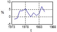
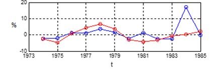
The Fig. 1 shows the changes in Germany’s economic indicator – OECD complex index of preliminary indicators (the Composite Leading Index) during the years 1962-1994 [22].

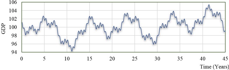
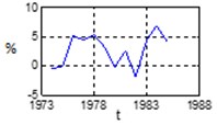
Having employed the possible parameters of the economic cycle elements (Table 1) in the Eq. (2), we get the graph of the long (Kondratjev) wave’s economic cycle (Fig. 2). The general semblance of the graph is qualitatively close to the real graph of the change in the economic indicator.

In this way, the general principles of the fluctuation theory may be applied to the research of the economic cycles. Vibrations in electronic, mechanic or other systems may be regarded as a suitable prototype when investigating fluctuations in biology, economics and similar fields.

On the other hand, different compound percentage is often employed when examining the economic processes. It appears that the widely used cumulative percentage is merely a separate case of the simple percentage. Let us now discuss the general forms of cumulative percentage.

Fig. 1The change in OECD complex index of preliminary indicators (the composite leading index)

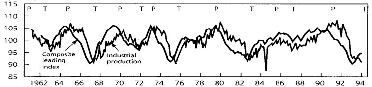
Fig. 2The economic cycle of one long (Kondratjev) wave, where A1= 0,5; A2= 1; A3= 2,3; A4= 1,4; A5= 1; T1= 0,6; T2= 2,6; T3= 9; T4= 20; T5= 45; φ1= 0,25; φ2= 1; φ3= 2; φ4= 0; φ5= 20; Kp=K0= 100, r= 1,03

3. General (logistic) cumulative percentage

It is clear that the percentage is not only a fraction, where the denominator is a hundred, but also a rule or a law of a certain value (over time). It is usually assumed that the rate is represented by two rules (over time) – a linear variation or an arithmetic progression (simple percentage) and an exponential variation or a geometric progression (compound or cumulative percentage). Therefore, the widespread simple and compound percentage represent growth rate. Compound percentage is called cumulative percentage due to their ability to cumulate interest. In this way the distinctive features of the cumulative percentage are that it exposes the growth (variation) of the population, is expressed by the initial population and percentage rate, and cumulates interest. Simple percentage is defined the same as cumulative, except that it does not cumulate the interest of the previous period. The sum which is paid for the use of the capital is called interest or simply percentage. It is important to note that a mere percentage formula (percentage model) is also often called percentage or interest.

Hence, rate is a certain rule for growth (cumulation). Yet, it may seem that such rules not necessarily are exceptional. When analyzing the growth phase of various populations, the conclusion was made that it is possible to employ other time functions which contains the values of the initial population and growth norm. Such functions fully meet the requirements for the simple and cumulative percentage. It is convenient to employ such values which are easy to transform into the shapes of simple or compound percentage.

It is important to stress that the rate types which were used up till now are of infinite growth. In reality, during the long period, the infinite growth does not exist as such. Experience has shown that each growth comes to an end sooner or later. Based on experience and phenomenological method it is possible to state that the rule for the infinite growth of the compound percentage should be substituted by the logistic function of the limited growth. It is recalled that the phenomenological method is in between the theory and experiment. In this case, the phenomenological method based on empirical evidence shows the limitation of the long-term growth. This fact is compatable with the fundamental theory of the logistic growth, though it is not extracted directly from it.

In the beginning of the 19th century, B. Gompertz [23] and Verhülst’s models were designed for the modelling of the limited growth. They employed the parameter of growth limit – the highest possible value of the product. We will call this value potential capital (potential product or potential population). Nevertheless, the models for the limited growth (logistic models) have not yet taken over compound and simple percentage.

When examining the growth of various populations, the application of logistic models is becoming more and more acceptable. When modelling the growth in different spheres of activity, different models are usually employed. In biology Verhülst’s model has been used for a long time, while in social science – F. Bass’s or B. Gompertz’s growth functions take precedence. However, the potential of the classical logistic models has not been harnessed enough yet, they were not employed for expressing the percentages. Moreover, the available models are not comfortable for the modelling of the economic dynamics. This is because the variables of these models are not expressed through the parameters of the percentage. Let us take the classical Verhülst’s model (Verhulst, 1838):

where $K\left(t\right)$ – the amount of the product (capital) per $t$ periods (sometimes instead of $K\left(t\right)$ we wil use $K$), $K_0$ – initial amount of the product, $K_p$ – potential (marginal, maximum) value of the product (capital) $t$ – duration (the number of periods), $m$ – coefficient, influencing the growth speed.

The essential step in the calculation of percentage has been taken when the general (logistic) percentage has been formed by applying the Eq. (3) (Girdzijauskas S. 2008). It has the following expression:

where $i=\mathrm{e}\mathrm{x}\mathrm{p}\mathrm{}\left(m\right)-1$ is growth (interest) rate, expressed by percentage for one time $t$ unit.

The trajectory for the general percentage is a logistic curve in the shape of an elongated letter “$S$”. The important aspect here is that, while the growth limit indefinitely increases, $\left(K_p\to \mathrm{\infty }\right)$, the Eq. (4) turns into a formula of compound percentage [4], i.e.:

Hence, we extract a well-known value of compound percentage out of logistic percentage Eq. (3):

Let us return to the Eq. (3). Here $K_p$ fixates growth limit, however the emphasis here is also placed on the ratio $K/K_p$ ($K<K_p$; $K\to K_p$). This ratio discloses the saturation level of the growth area. The saturation is an important aspect in biology, chemistry, physics and other areas of science. The research has shown that in economics this fact is significant, even essential. In economics it usually reveals itself as market saturation. Market saturation is defined as partial or complete filling (completion) of the closed or partially closed market by the capital. It reveals itself as the excess (overproduction) of certain market products. Market saturation begins when market capacity from infinite turns into measurable, or when the investment is faster than the expansion of the market itself (when the demand grows faster than the supply) [5].

When modelling the growth with logistic interest Eq. (4), it was noticed that the increased saturation (when the growth comes to a point of saturation, i.e. when $K/K_p\to$1) results in the increasement of the internal rate of return. This is a particularly important fact when considering market saturation by capital and overproduction.

4. The transformation of the logistic model. Calculation of the typical duration

The following chapter will deal with reorganization of statistical data, the possibilities for their transformation. There exist various modes of transformation. In our case, rectilinear transformation is related with the reorganization of logistic functions and statistical data. For this we will apply Fisher-Pry transformation [24]. For the calculation of the growth parameter, the truncated mean will be used. Such mean is calculated not from the whole rank order but from its central part, which is obtained by rejecting the same number of the lowest and highest values of the attribute (e.g. a truncated mean of 80 % is calculated by rejecting 10 % of the lowest and 10 % of the highest values of the sample). For this reason the truncated mean is considerably more resistant to the influence of extreme values, and is used when these values seem unreliable. In the case of economic markets, extreme values may be formed as a result of the heating market [1].

For this reason we will extract independent variable time $t$ from the Eq. (4):

In the Eq. (5), the size of the capital may be expressed as a part of the potential product $K_p$_. The growth period in the model may be called a typical duration and marked as $\mathrm{\Delta }t$. When the trajectory grows from 10 % to 90 % of the potential capital $K_p$ value, $\mathrm{\Delta }t$ will be:

i.e:

It is convenient to use the parameter $\mathrm{\Delta }t$ when analyzing the data of the historic time series. When considering other boundaries of trajectory change than we did before, the parameter $\mathrm{\Delta }t$ will be shaped differently. From the Eq. (6) we get the following value:

If this value is incorporated into the logistic interest Eq. (4) and supposing that $K_0=\text{0.1}{K}_p$ ($K_0$ we identify as the bottom value of the interval), we come across a new value of the growth model:

The main advantage of this model is that there is smaller amount of variables – instead of the value $K_0$, only $\mathrm{\Delta }t$ is left. Moreover, the results of the analysis are of greater precision – by eliminating the highest and lowest values of the statistical data, the distortion of the possible forecasting is reduced.

5. Logistic growth modeling method

Frequently, classical growth models are applied to solve relevant problems of modeling product growth. Evaluation of market capacity $K_p$, is one of the most problematic tasks of modeling. Logistic model is able to detect unusual cases and unsustainable growth stages. Applying digital methods and fuzzy logic with transformed interval logistic model increases the accuracy of results [25].

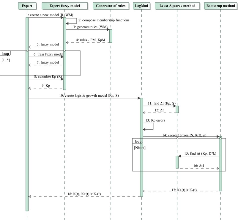
In the following chapter modeling with transformed interval logistic model Eq. (7) will be presented. All modeling mechanism consists of: expert fuzzy system (used to calculate $K_p$, the value of market saturation parameter), generator of the rules, transformed interval logistic model, the least squares and bootstrap methods, it also includes the principle of errors calculation (Fig. 3).

In Fig. 3 one of the main roles in the given diagram of sequences is undertaken by a highly qualified expert of the market. He specifies influencing parameters of appropriate market. Generator of the rules, regarding parameters weights which are provided by the expert, generates rules which are used in fuzzy system. In the fuzzy system calibrated membership functions have to satisfy initially raised requirements. The composed expert model forecasts $K_p$(saturation parameter). When we determined $K_p$ value of logistic growth model, then second parameter $\mathrm{\Delta }t$ is discovered by applying least squares method, and we also define percentage errors for $K_p$ parameter. The bootstrap method corrects errors of predicted saturation parameter $K_p$. Expert evaluates the received results and decides if this model correctly predicts saturation parameter. [26].

Least squares method is applied to attract the statistical points to the mathematical function. In present case the least squares method expression is:

By applying this method with the saturation value $K_p$ the second parameter $\mathrm{\Delta }t$ of the interval logistic growth model is discovered [26].

Populating created expert fuzzy model, additional percentage error: $K_p^{+}$ ir $K_p^{-}$ (positive and negative increment) are introduced to predict the parameter $K_p$. Mathematical expression looks like this, where error $p\in \left(\text{0, 1}\right)$ [26]:

In this way the interval $t$ in time moment of predicted parameter $K_p$ is between $K_p^{-}$ ir $K_p^{+}$ [26]:

Fig. 3Simulation sequence diagram

The method of least squares is applied to functions $K^{+}\left(t\right)$ and $K^{-}\left(t\right)$ with the same statistical points. With new $K_p$ values unknown variables ${∆t}^{+}$ ir ${∆t}^{-}$ computed.

Sometimes it is not just enough to evaluate standart error. Therefore boostrap principle is used as alternative to traditional approach, which was introduced by Efron B. in 1979. Bootstrap method is used to evaluate how accurate are the results of least square method [27].

Set of errors $P$ is given from difference of statistical and logistical values in appropriate time moment $t$. From given error collection (original set) at random a set of errors $P^{*}$ is pulled with recurrence, here size of sets is the same. Based on this set a new statistical data set $D^{*}k$ is formed:

$D_k^{*}=K\left(t,∆t_0\right)+P^{*}$, where $\mathrm{\Delta }{t}_0$ – value founded by least squares method ($=\mathrm{\Delta }t$). With the new data set $D^{*}$ new $\mathrm{\Delta }{t}^{*}$ value is calculated using least squares method. Creation of new statistical data sets and new $\mathrm{\Delta }{t}^{*}$ calculations are reaped $N_{boot}$ times. $N_{boot}$ is an integer, greater than 0 number, which is chosen freely. Now new $\mathrm{\Delta }T$ set is created from found $\mathrm{\Delta }{t}^{*}$ values. Confidence interval CI (5 % and 95 % percentage) is marked on the histogram build from $\mathrm{\Delta }T$. The method is applied to $K^{+}\left(t\right)$ and $K^{-}\left(t\right)$ functions. In case of$K^{+}\left(t\right)$ we take 5 % percent value, and $K^{-}\left(t\right)$ we take 95 % percent. Thus forecast saturation parameter’s $K_p$ error in the transformed logistic model is corrected using “Bootstrap” method [26].

6. The examination of the real estate market index in the USA

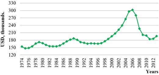
Modeling mechanism is performed with a realistic example of USA real estate market to calculate saturation. The given graph (Fig. 4) demonstrates that USA market of real estate has suffered three economic declines: 1974-1985 years, 1983-1992 years and 1996-2013 years [28].

Fig. 4Data of real estate market in the USA

The expert has chosen the following four parameters typical to the USA market which affect growth: national average wages (NAW), state‘s GDP, current unemployment rate (CUR) and consumer price index (CPI) [29, 30].

Parameter set is defined like this:

For defined USA market economical parameters are given weights: $W_e=$ {0.3, 0.3, 0.1, 0.3} accordingly.

Following the given methodology (Fig. 5) the fuzzy expert model is created for the case of USA real estate market. $K_p$ dinamic of saturation in time moment $t$ is shown in Fig. 6, which is created (trained in the fuzzy system) according to the data of the first USA real market crisis period (1974-1985 years) [26].

Fig. 5Statistical parameters – NAW, GDP, CUR, CPI variability – fuzzy expert system Kp changes forecast

a) NAW

b) GDP

c) CUR

d) CPI

e)$K_p$

Every crisis period model had shown deviation from the correct growth, warning of instability. Below is presented the forecast saturation result of third period. It is worth noticing USA real estate market index growth deflection which warns about third bubble formation and the impending threat. The third crisis was in 2006-2007 years.

The graphs show modeling results. For modeling 1994-2013 period data is used. In the 1994-1997 period a slight fluctuation is visible [26].

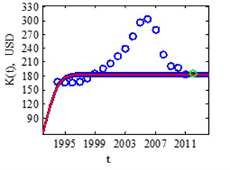
In 1998 year noticeable first deviation from growth function. Fig. 6 shows the deviation from forecasted growth in 1998 and 1999.

Fig. 6USA real market saturation assessment in 1998 and 1999 years

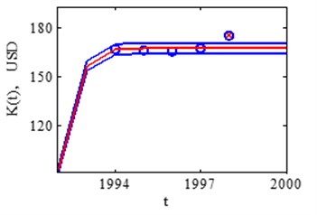
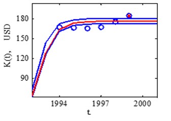
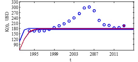
Fig. 7USA real market saturation assessment in 2006 and 2012 years

In 2000-2005 the model shows discrepancy from normal growth line, no actions were taken to suppress the growth, that is why in 2006 occurs bubble burst (Fig. 7), and this causes the fall in year 2007.

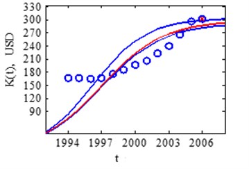
Fig. 8USA real market saturation assessment in 2013 year

The growth falls from years 2007 to 2011. In the 2012 were positive increase, but in 2013 model shows visible growth discrepancy (Fig. 8). When market was stabilized, the model shows, growth again going too fast. It is necessary to look at market economic parameters growth and their dynamics. It is appropriate to suppress rapid market growth, otherwise it is likely that 4th USA real market growth recession will happen [26].

In summary of the modeling process we can state, that the model is able to recognize upcoming recession threat, identify economic bubble formation period.

7. Conclusions

Economic fluctuations form a distinct part in the area of common fluctuations. General principles of the fluctuations theory are applied to the research of the dynamics of the economic cycles.

After applying the phenomenological method, examining the structure of the well-known logistic models and investigating their mathematics, it is fair to claim that the logistic models are suitable for the modelling of the economic issues, since it is possible to express the growth parameter through the interest rate by employing the special substitution.

Having examined the cases of the limited growth, having compared reorganized logistic models and having employed phenomenological method, a model of general interest has been found. The model of general interest permits to comprehensively examine any growth process and to consider its cyclical variations.

The advantages and potential of general (logistic) rate have been identified. Logistic rate model highlights the specifics of growth dynamics and at the same time contributes to the disclosure of the unknown economic paradoxes.

Based on newly created method provides an opportunity to investigate market heating, formation of financial bubbles, and recognize an approaching decline and unstable market situations. Error correction of saturation parameter $K_p$ gives more accurate final result. Consumer can take appropriate economic and management actions to prevent crisis.

For USA real estate market index a trustworthy fuzzy model is created. It is showed, that model can be used to recognize upcoming growth recession threat, when training was accomplished by first bubble formation period. Is necessary to make proper conclusions and perform right actions to suppress uncontrolled growth as early as possible, so that recession consequence will be minimal.