A comparison study on application of model reduction methods in rotor dynamics

Wang, Fei; Luo, Guihuo

Vibroengineering Procedia

Browse Procedia

Published: 18 September 2015

Check for updates

A comparison study on application of model reduction methods in rotor dynamics

Fei Wang¹

Guihuo Luo²

^{1, 2}Nanjing University of Aeronautics and Astronautics, College of Energy and Power Engineering, Nanjing 210016, China

Corresponding Author:

Guihuo Luo

Cite the article Download PDF

Downloads 1358

Abstract

To reduce computation effort, model reduction technique has been widely used in rotor dynamics. In this paper, different model reduction methods, including Guyan reduction, dynamic reduction, improved reduction system (IRS), System equivalent expansion reduction process (SEREP) and component modal synthesis method (CMS), were introduced and compared. All methods were applied to a single rotor system to obtain the critical speeds. By the eigenfrequencies comparison and the MAC comparison, it was found that CMS was the most convenient reduction method for rotor dynamics.

1. Introduction

Model reduction is an important issue in rotor dynamics. For the constant demand of working with increasingly large models while aiming to control and possibly reduce storage and simulation time needs, the application of the reduction method constitutes an important decision.

A common spatial discretization method used for rotor system analysis is the finite element method. The equations of motion of a rotor system are second order ordinary differential equations (ODE) which are of the form:

1

M \ddot{q} (t) + C \dot{q} (t) + K q (t) = f (t),

where $M,$ $C,$ $K \in R^{n \times n}$ are the system matrices (inertia, damping and stiffness matrix respectively). $f (t) \in R^{n \times 1}$ , the load vector and $q \in R^{n \times 1}$ the unknown vector of degrees of freedom (DOFs).

The general concepts of model reduction is to find a low-dimensional subspace $T \in R^{n \times n}$ in order to approximate the state vector $q = T q_{r} + ε$ . By projecting Eq. (1) on this subspace a lower dimension 2nd-order ODE is obtained:

2

M_{r} {\ddot{q}}_{r} (t) + C_{r} {\dot{q}}_{r} (t) + K_{r} q_{r} (t) = f_{r} (t),

where $M_{r} = T^{T} M T,$ $C_{r} = T^{T} C T,$ $K_{r} = T^{T} K T$ being the reduced system matrices and $f_{r} (t) = T^{T} f (t)$ the reduced load vector. The effectiveness and reliability of the reduction method depends on the size of $ε$ . Based on the choice of $T$ , different reduction techniques have been developed in the last decades.

2. Model reduction methods

2.1. Guyan reduction

Guyan reduction method [1] is one of the oldest and most popular reduction method, also called static reduction method, where the inertia and damping terms associated with the discarded degrees of freedom are neglected.

Assuming the damping is negligible, the partitioned equations of motion can be written as:

3

[\begin{matrix} M_{m m} & M_{m s} \\ M_{s m} & M_{s s} \end{matrix}] [\begin{matrix} {\ddot{q}}_{m} \\ {\ddot{q}}_{s} \end{matrix}] + [\begin{matrix} K_{m m} & K_{m s} \\ K_{s m} & K_{s s} \end{matrix}] [\begin{matrix} q_{m} \\ q_{s} \end{matrix}] = [\begin{matrix} f_{m} (t) \\ 0 \end{matrix}] .

The subscripts $m$ and $s$ relates to the master and slave coordinates respectively. Neglecting the inertia terms in the second set of equations the slave degrees of freedom can be eliminated:

4

{[\begin{array}{l} q_{m} & q_{s} \end{array}]}^{T} = {[\begin{array}{l} I & - K_{s m}^{- 1} K_{s s} \end{array}]}^{T} [q_{m}] = T_{s} q_{m},

where $T_{s}$ denotes the static transformation between the full state vector and the master coordinates.

The reduced mass and stiffness matrices are then given by:

5

M_{R} = T_{s}^{T} M T_{s}, K_{R} = T_{s}^{T} K T_{s} .

Generally, Guyan reduction is a good approximation for the lower eigenvalues, in fact it is exact only at zero frequency. For high frequency motion, the effect of inertia terms is significant, thus the method becomes inaccurate.

2.2. Dynamic reduction

The dynamic reduction [2] is an alternative or expansion of the static reduction, where the frequency at which the reduction is exact may be chosen arbitrarily. Suppose the reduction is to be exact at $ω_{0}$ , then approximation of the inertia forces for the second set of equations in Eq. (3) can be expressed as:

6

F_{i n e r t i a} = - ω_{0}^{2} [\begin{array}{l} M_{s m} & M_{s s} \end{array}] {[\begin{array}{l} q_{m} & q_{s} \end{array}]}^{T} .

So the reduction transformation can be written as:

7

{[\begin{array}{l} q_{m} & q_{s} \end{array}]}^{T} = [\begin{matrix} I \\ - {[K_{s s} - ω_{0}^{2} M_{s s}]}^{- 1} [K_{s m} - ω_{0}^{2} M_{s s}] \end{matrix}] [q_{m}] = T_{d} q_{m} .

Dynamic reduction approximates better high-frequency motion than Guyan reduction. However the dependence of $T_{d}$ on $ω_{0}$ constitutes the choice of an appropriate initial frequency, which is not a trivial task.

2.3. Improved reduction system method (IRS)

The improved Reduction method is proposed by O’CALLHAN [3]. In this approach, an extra term is added to the static reduction transformation to make allowance for the inertia forces. This inertia term allows the modal vectors of interest in the full model to be approximated more accurately but relies on the statically reduced model.

By binomial theorem, Gordis [4] derived the transformation matrix for the IRS method. For a given frequency $ω$ , from Eq. (3):

8

[K_{s s} - ω^{2} M_{s s}] q_{s} = - [K_{s m} - ω^{2} M_{s m}] q_{m},

which is quite similar to Eq. (7).

By neglecting the error and considering that the IRS method is based on the static reduction method, rearranging Eq. (8) gives:

9

T_{I R S} = T_{s t a t i c} + [\begin{array}{l} 0 & 0 \\ 0 & K_{s s}^{- 1} \end{array}] M T_{s t a t i c} M_{R}^{- 1} K_{R} .

With Eq. (9), it is convenient to calculate the transformation matrix of IRS method. Because all notations in the equation can be obtained from previously described Guyan Reduction method.

2.4. System equivalent expansion reduction process

There are many reduction methods in which the subset of the eigenvectors are utilized. Let the subset be $Φ_{r}$ , transformation matrix can be written as $T = Φ_{r}$ . With this transformation, the physical coordinates are transformed into modal coordinates. System equivalent expansion reduction process (SEREP) [5] also adopts the subset of the eigenvectors. However the physical coordinates are retained by partitioning both the physical coordinates and the eigenvectors with master DOFs and slave DOFS. The transformation can be written as:

10

{[\begin{array}{l} q_{m} & q_{s} \end{array}]}^{T} = {[\begin{array}{l} Φ_{m} & Φ_{s} \end{array}]}^{T} Φ_{m}^{- 1} q_{m},

where $Φ_{r} = {[\begin{array}{l} Φ_{m} & Φ_{s} \end{array}]}^{T}$ denotes the partitioned subset of the eigenvectors.

So the transformation matrix:

11

T_{S E R E P} = {[\begin{array}{l} Φ_{m} & Φ_{s} \end{array}]}^{T} Φ_{m}^{- 1} .

To obtain this transformation matrix, eigenvectors of the undammed system must be calculated first. After that, $T_{S E R E P}$ and the reduced mass and stiffness matrice can be calculated.

Compared to dynamic reduction and static reduction, SEREP predict better high frequency motion of the system up to the predefined limit.

2.5. Component mode synthesis method (CMS)

The component mode synthesis method was proposed by Craig and Bampton in 1968 [6] and were further developed by Craig and Petyt [7-10] et al. Fixed interface and free interface CMS were developed. In this paper, only the fixed interface CMS is introduced.

To apply CMS, the structure is divided into substructures which consist of the interface or external substructures and the internal substructures. According to the division, the physical coordinates can be partitioned into external and internal coordinates corresponding to the previously described master and slave DOFs.

Analogue to Eqs. (3) and (4), the constraint mode of CMS can be determined by:

12

0 = K_{s m} q_{m} + K_{s s} q_{s} or q_{s} = - K_{_{s s}}^{- 1} K_{s m} q_{m} = Φ_{c} q_{m} .

And $Φ_{c}$ is the desired constraint mode. Also the normal modes or the Craig-Bampton modes should be calculated with the following equation:

13

K_{s s} Φ = λ M_{s s} Φ,

where $Φ$ denotes the eigenvector, $λ$ the eigenvalue. $Φ$ can be truncated to neglect the high order frequencies, the truncated eigenvector is expressed with $Φ_{r}$ .

Finally, with basic assumption by Craig and Bampton, the displacement of the slave coordinates is given by:

14

q_{s} = Φ_{c} q_{m} + Φ_{r} y .

Thus, the transformation is:

15

[\begin{matrix} q_{m} \\ q_{s} \end{matrix}] = T_{C M S} [\begin{matrix} q_{m} \\ y \end{matrix}] and T_{C M S} = [\begin{matrix} I & 0 \\ Φ_{c} & Φ_{r} \end{matrix}] .

Just like other reduction methods, CMS has its own advantages and disadvantages. It approximates good results of the reduced structure. But the high order terms of the normal mode are neglected which might increase the inaccuracy of the prediction results.

3. Numerical solution and results comparison

3.1. Model of the rotor system

A shaft-line model of a single rotor system is established with the finite element method, in which the Timoshenko beam element is adopted. Both the damping and internal friction are neglected. The model consists of 21 elements, 22 nodes and 88 DOFs. The schematic and bearing locations of the model are shown in Fig. 1.

Fig. 1Schematic of the single rotor system

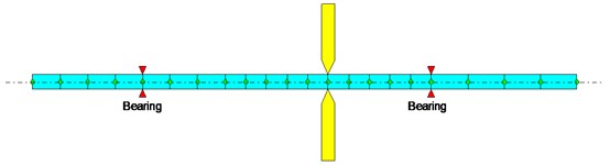
For this rotor system, DOFs related to nodes 1, 5, 13, 18, 22 are selected as master DOFs for Guyan reduction, Dynamic reduction, IRS and SEREP. As for the CMS, only the DOFs related with nodes 5 and 13 are selected as master DOFs.

3.2. Results

For all reduced models and the full model, eigenvalues and eigenvectors as well as the Campell diagram are calculated. The Campell diagram calculated with full model as well as eigenfrequencies comparison between different methods are shown in Fig. 2. Slight differences do exist between results calculated by different methods. All results are listed in Table 1.

Differences of eigenfrequencies are defined as:

16

e i g_{d i f f} = e i g_{r e d u c e d} - e i g_{f u l l} .

Fig. 2Campell Diagrams and eigenfrequency comparison

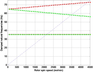
a) Campell diagram for full model (forward whirl is red, backward whirl is green)

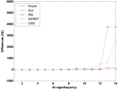
b) Eigenfrequency comparison

From Table 1 it can be seen that the dynamic reduction method predict better 1st forward and backward critical speeds than Guyan reduction method and this is due to the appropriate selection of $ω_{0}$ in Eq. (7). In this case, $ω_{0} =$ 220 rad/s $\approx$ 35 Hz. Also from Table 1, the IRS method and SEREP method predict accurate results comparing with that calculated with the full model.

To evaluate correlations between full model and the reduced models, modal assurance criterion [11] was calculated.

Table 1Critical speed comparison

Critical speed (Hz)	Full	Guyan	Dynamic	IRS	SEREP	CMS
1st backward	35.5424	35.5434	35.5424	35.5424	35.5424	35.5243
1st forward	35.5043	35.5053	35.5043	35.5043	35.5043	35.5425
2nd backward	58.2077	58.2177	58.2118	58.2078	58.2077	58.2082
2nd forward	72.7526	72.7818	72.7698	72.7528	72.7526	72.7540

Fig. 3MAC Comparison

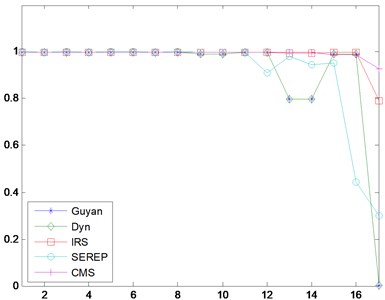
a) MAC Comparison-All Methods

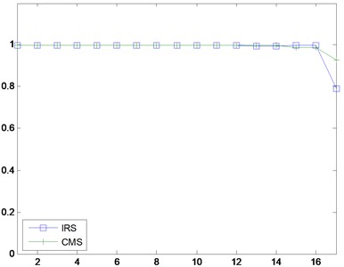
b) MAC Comparison –IRS and CMS

As indicated by Fig. 3(a) and (b), the Guyan reduction method and dynamic reduction method are identical, IRS and CMS correlates better with the full model comparing with other three methods. The MAC comparison results coincides with that of eigenfrequencies.

4. Conclusions

Different model reduction methods are compared. Comparison for differences of eigenfrequencies implies that IRS and CMS deliver the best eigenfrequency results. Guyan reduction is the most unreliable and least efficient method because of its static nature which means it’s only exact at zero frequency. The differences between Guyan reduction and dynamic reduction lie in that the dynamic reduction can be exact at the chosen frequency instead of zero frequency. However, it is not a trivial task to choose the appropriate frequency.

The SEREP method is better than Guyan reduction and dynamic reduction in accuracy although when predicting high frequency motion it is less accurate and less efficient than the CMS and IRS method.

The CMS and IRS methods are almost equivalent in approximating the simple rotor system adopted in this paper. Still the CMS method has better accuracy in predicting high frequency motion. Besides, CMS is advantageous to deal with time series analysis of high-dimension nonlinear rotor systems which are discussed in references [12-14] in which the nonlinear rotor system is modeled and analyzed with free interface mode synthesis method. The IRS method is extended by M. I. Friswell [15] and called the iterated IRS method which has a better accuracy in predicting high frequency motion. However, the increased accuracy of the reduced model is always gained at the expense of increased computation.

References

Guyan J. Reduction of stiffness and mass matrices. AIAA, Vol. 3, 1965.

Search CrossRef
Paz Mario Dynamic condensation. AIAA, Vol. 22, Issue 5, 1984, p. 724-727.

Search CrossRef
O’Callhan J. C. A procedure for an improved reduced system (IRS) model. Proceedings of the 7th International Modal Analysis Conference, Las Vegas, 1989, p. 17-21.

Search CrossRef
Gordis Joshua H. An analysis of the improved reduced system (IRS) model reduction procedure. International Modal Analysis Conference, Vol. 1, 1992, p. 471-479.

Search CrossRef
Sastry C. V. S., Mahapatra D. Roy, Gopalakrishnan S. An iterative system equivalent reduction expansion process for extraction of high frequency response from reduced order finite element model. Computer Methods in Applied Mechanics and Engineering, Vol. 192, Issue 15, 2003, p. 1821-1840.

Search CrossRef
Craig R., Bampton M. Coupling of substructures in dynamic analysis. AIAA, Vol. 6, 1968.

Search CrossRef
Craig R. Coupling of substructures for dynamic analyses: an overview. AIAA, 2000.

Search CrossRef
Craig R., Chang C. J. Free-interface methods of substructure coupling for dynamic analysis. AIAA, Vol. 12, 1976.

Search CrossRef
Rixen Daniel A dual Crai-Bampton method for dynamic substructuring. Journal of Computational and Applied Mathematics, Vol. 168, Issues 1-2, 2004, p. 383-391.

Search CrossRef
Rixen Daniel, Farhat Charbel, Géradin Michel A two-step, two-field hybrid method for the static and dynamic analysis of substructure problems with conforming and non-conforming interfaces. Computer Methods in Applied Mechanics and Engineering, Vol. 154, Issues 3-4, 1998, p. 229-264.

Search CrossRef
Randall J. A. The modal assurance criterion-twenty years of use and abuse. Sound and Vibration, 2003, p. 14-20.

Search CrossRef
Huang Taiping, Luo Guihuo Rotordynamics optimization. Journal of aerospace power, Vol. 9, Issue 2, 1994, p. 113-116, (in Chinese).

Search CrossRef
Yang Xiguan, Luo Guihuo, et al. Acceleration response characteristics of a counter-rotating dual rotor system. Journal of Vibration and Shock, Vol. 33, Issue 2, 2014, p. 105-111, (in Chinese).

Search CrossRef
Yang Xiguan, Luo Guihuo, et al. Modeling method and dynamic characteristics of high-dimensional counter-rotating dual rotor system. Journal of Aerospace Power, Vol. 29, Issue 3, 2014, p. 585-595, (in Chinese).

Search CrossRef
Friswell M. I., Garvey S. D., Penny J. E. T. Model reduction using dynamic and iterated IRS techniques. Journal of Sound and Vibration, Vol. 186, 1995, p. 311-323.

Search CrossRef

About this article

Received

Accepted

28 August 2015

Published

18 September 2015

SUBJECTS

Mechanical vibrations and applications

Keywords

model reduction

rotor dynamics

component mode synthesis method

improved reduction system

This is an open access article distributed under the Creative Commons Attribution License, which permits unrestricted use, distribution, and reproduction in any medium, provided the original work is properly cited.