Seismic signals discrimination based on instantaneous frequency

1. Introduction

Clustering of seismic signal is one of the key problems in seismic signals analysis. Such clusters could contain signals representing different source mechanisms, seismic source locations, seismic moment, slip direction, energy of the seismic event, blasting with different blasting techniques etc. When the entire seismic catalogue is divided into clusters, one can perform root-cause analysis taking into account a specific kind of seismic signals only. The crucial step in clustering is to define a rule (criterion) which distinguishes the seismic signals. A good criterion is expected not only to differentiate two signals from different clusters, but also to equate two signals from the same cluster. Such criteria are based mainly on the P-wave arrival analysis, ratio between P- and S-wave amplitudes, frequency content of the signal etc. In this paper we investigate instantaneous frequency (IF) as a basis for a criterion distinguishing seismic signals.

Instantaneous Frequency of a signal is very practical feature which proved its usefulness in wide range of scientific fields (e.g. financial time series analysis [1], machine health monitoring [2], earthquake analysis [3]). It may be interpreted as the frequency of a sine wave which locally fits the analyzed signal. In order to calculate IF of a signal, it has to be ensured that the signal is a monocomponent. Otherwise, IF calculates an instantaneous frequency of a signal, but there is no information about which component reveals such frequency at a given time point. Moreover, there might be even no component in the raw signal with such instantaneous frequency. IF is strictly related to the frequency modulation. If a sine wave is frequency modulated, one can notice a set of sidebands around the carrier frequency in the amplitude spectrum. Such set of sidebands is related to a Bessel function with appropriate $\alpha$ [4]. Thus, one can obtain a monocomponent signal by bandpass filtering around the carrier frequency with appropriate bandwidth. If the desired bandwidth is too wide, one can expect other components in this frequency band. Thus, if carriers of two components of the raw signal are close to each other, it makes obtaining a monocomponent a very challenging problem. Another way of obtaining a monocomponent signal is based on Empirical Mode Decomposition (EMD). This method iteratively decomposes the raw signal into a sum of so called Intrinsic Mode Functions (IMFs) and a Residuum. The number of IMFs depends on the considered signal. Each of the IMFs might be considered as a monocomponent, thus they can be a basis for IF calculation. Such method of obtaining IF using EMD is called the Hilbert-Huang transform [5]. EMD requires no assumptions of input data thus it is a great tool to analyze nonstationary series (as in the case of seismic vibration signals). It has found its application in several fields, e.g. rotating machinery diagnostics [6], speech signals processing [7], medicine [8], navigation [9]. EMD is not only procedure of receiving monocomponents – it is also often used for smoothing the signal when first IMFs contain noisy signals [10].

2. Seismic data description

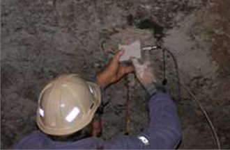
In this paper we analyze seismic vibration signals acquired using a sensor independent to the commercial seismic system installed in the underground copper ore mine. The sensor is a triaxial accelerometer mounted on the mining corridor roof using gypsum binder (Fig. 1). Range of sensor is 0.001-100 m/s², frequency range is 0.5-400 Hz and sampling frequency is set to 1250 Hz. At the beginning of the experiment, the distance between the sensor and the mining face was 20 m, but it increased to 140 m due to advance of mining works. Due to the quality of the seismic vibration signals acquired during this experiment, the level of noise is relatively low. There is no distortion in industrial electrical network. In this paper we analyze 51 seismic recordings which are segmented into 98 signals (segments), each consists of one seismic event. The segmentation procedure is based on time-frequency analysis and is focused on detection of significant changes of the amplitude spectrum. Moreover, this procedure trims the signals, thus signal portions with near-zero amplitude are cutoff.

Fig. 1The accelerometer located on the mining corridor roof

3. Methodology

In this section we present how to derive a powerful IF-based criteria for seismic vibration signals clustering. At first, monocomponents from each of 98 signals have to be derived using EMD. In our preliminary study we consider the first IMF only. Kaslovsky and Meyer in [11] highlighted, that couple of first IMFs could contain noise, thus they should not be included in IF analysis. Although, in our case the signal is not affected by significant amount of noise (Fig. 2), so the first IMF might be considered as a monocomponent signal with meaningful instantaneous frequency. IF calculated from the first IMF constitutes a basis for two criteria for seismic signals discrimination.

3.1. Distribution of instantaneous frequency

The first criterion is designed to provide limited information about variation of the IF in time. Moreover, it provides the same size of parameters for signals of different duration. To wit, our criterion is a probability density function (PDF) estimator which quantifies probability of IF presence at a given frequency during the entire signal. As a PDF estimator we use the Rozenblatt-Parzen kernel density estimator with Gaussian kernel [12, 13]. Such density gives information about behavior of IF through the entire signal. If the IF does not significantly change in time, the density should form a spiky bell-shaped curve. If the IF switches between two or more main frequencies, the density should indicate a bi- or multi-modal distribution. Chirp-like signals should be indicated as a wide bell-shaped curve. Probability of each mode indicates percentage time during which the IF occupied given frequency.

Fig. 2Typical recording of a seismic event

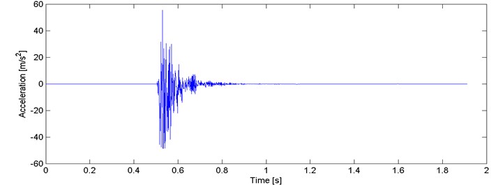
Fig. 3Probability density function estimators for all segments

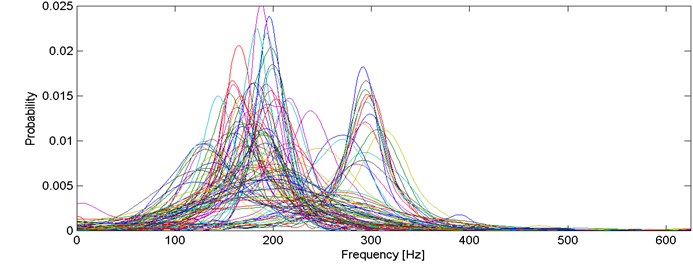
As it can be seen in Fig. 3, one can identify a few clusters. The first one consists of unimodal bell-shaped curves with relatively low dispersion. Modes of these IF distributions are located approx. at 300 Hz and probabilities vary from 0.01 to 0.02. There are also several narrow bell-shaped densities with modes located slightly below 200 Hz (probability 0.15-0.25). One can notice also wide bell-shaped curves with modes at about 130 Hz and with probability 0.01.

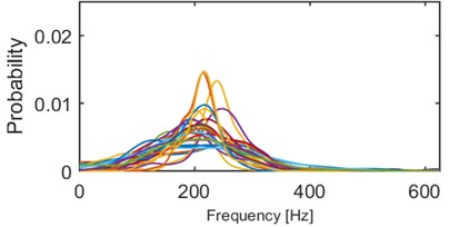
We performed series of clustering with different numbers of clusters using the $k$-means method [14]. It minimizes the total intra-cluster variance using a heuristic algorithm [15]. It has been noticed that 5 clusters seems to provide the best results, i.e. densities within a single cluster are similar to each other and each two densities from different clusters might be easily distinguished. Obviously, some outliers can be noticed e.g. modes of 2 densities in cluster 2/5 (Fig. 4) are outlying – their modes are close to 0.015, but the average mode is close to 0.01. Such behavior might be caused by the segmentation procedure which might be imperfect (e.g. one segment containing more than one seismic event). Moreover, heuristic $k$-means algorithm might misclassify single densities. Although, the result presented in Fig. 4 clearly indicates a well-behavior of the proposed criterion. Instantaneous frequency distributions contained in the 1st and 4th clusters oscillate around 200 Hz, however plots in the 4th one is much more flat, i.e. dispersion of IFs from the first IMF is much larger therein. Dispersions of 3rd and 5th clusters are comparable, however they are differ in terms of mean or mode location (300 Hz and 170 Hz, respectively). Mean of probabilities from the 2nd set is the lowest (~130 Hz). Moreover, several probability density function estimators seem to be bi- or multi-modal. To sum up, densities within clusters are similar to each other, except a few outlying or misclassified ones. When representatives of different clusters are compared, they are significantly different in terms of mean, mode, location of the mode, dispersion, the number of modes etc. Clear discrimination between the clusters is one of the main advantages of this criterion. On the other hand, the number of parameters (512) might cause problems in terms of computational complexity.

Fig. 4Results of clustering using IF density estimator – 98 segments partitioned into 5 clusters

a) Probability of frequency (cluster 1/5)

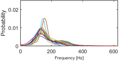
b) Probability of frequency (cluster 2/5)

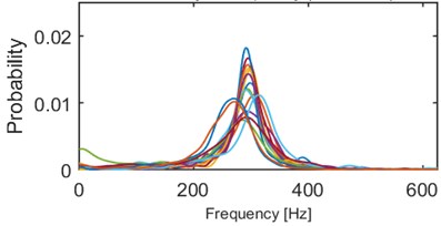
c) Probability of frequency (cluster 3/5)

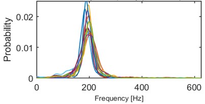
d) Probability of frequency (cluster 4/5)

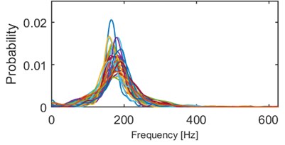
e) Probability of frequency (cluster 5/5)

3.2. Mode of a frequency

Our second criterion provides a limited information contained in the previous one. We propose to distinguish the signals by mode of frequency, at which the probability density function reaches its maximum. Therefore, each of 98 segments is represented by a single value between 0 and 625 Hz (Fig. 5).

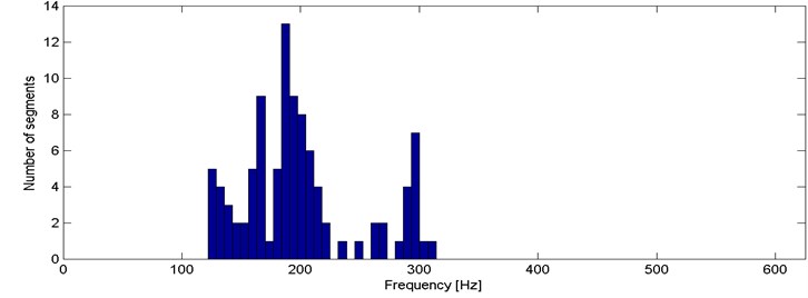
By analyzing Fig. 5 we can identify that for several segments the mode is located close to 300 Hz and they are clearly separated from the rest of the segments. However, is difficult to distinguish more sets with specific dominating value of the criterion. In order to check if other dominating criterion values might be separated, we plot a histogram (Fig. 6).

One can easily notice 4 dominating modes, i.e. close to 130, 170, 200 and 300 Hz. The results are intuitive considering outcomes of the first criterion (section 3.1.). Segments from 1st and 4th cluster obtained using the first criterion has been merged into a single cluster (near 200 Hz). 6 segments between 200 Hz and 300 Hz are identified as the outliers (in terms of mode) in the 1st and 3rd cluster from criterion in section 3.1. Recall, that the previous criterion consists of 512 parameters quantifying probability with respect to frequency. The location of the mode is just a single parameter, thus one can benefit from it when a computationally expensive algorithm is used for clustering. Moreover, one dimensional parameter makes possible to take advantages from sorting the data before clustering.

Fig. 5Location of the mode for all segments

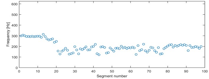
Fig. 6Histogram of 2nd criterion values

4. Conclusions

In this paper we proposed two different approaches to problem of analyzing similarities of seismic signals. These criteria divide the set of 98 segments into 4 or 5 clusters with similar properties within a single cluster and different between clusters. Both of the criteria incorporate empirical mode decomposition in order to obtain instantaneous frequency. One of the criteria quantifies the time-varying nature of the IF and the second one “compresses” it by providing only a single parameter instead of 512 parameters. It is beneficial for further clustering in terms of computational time.

However, when the criterion becomes one-dimensional (like the second one), it is much simpler to answer whether or not two events are similar. On the other hand, the multidimensional criterion (like the first one) provides more information about each seismic record.

It is worth mentioning that there are several methods that indicate the optimal amount of clusters. In this paper the number of clusters has been chosen arbitrary, thus an investigation on such criteria might resolve this problem.