Differences in time-varying group delay of seismic signals

1. Introduction

The problem of distinguishing between different seismic events is a critical issue of seismic vibration signal processing. Seismic monitoring systems in underground mines are often equipped with procedures for localization and quantification of energy. Such information might predetermine seismic hazard maps. Although, not every seismic event should be considered in such analysis. For instance, some seismic events might be caused by blasting, thus they are predictable and depend on the technology used in a particular mine. In the literature one can find several approaches to dealing with discrimination of seismic events. They are based mostly on arrivals of P-waves, ratio of P- and S-wave amplitudes, repetition of subsequent events etc. [1-4]. In this paper we propose to incorporate autoregressive modeling of the seismic signals using sliding-window AR model. Properties extracted from such model might provide information regarding the entire course of the seismic event.

Analysis of amplitude response of the instantaneous AR model has found application in several fields where non-stationary signal are considered, e.g. rotating machinery diagnostics and structural health monitoring [5-9]. Amplitude response (called ARgram [10]) of such model is an alternative to the classical spectrogram. Although, amplitude response is just one of the properties of the model – phase and phase-related characteristics might extend information about the fitted model and, therefore, about the seismic event. Therefore, we are looking for an attribute which can identify differences between examined signals, which cannot be distinguished using amplitude response. A promising solution might be to analyze a seismic signals using a sliding-window autoregressive model and investigate volatility of coefficients in terms of group delay – derivative of phase spectrum with respect to frequency.

The group delay of signal is widely used in speech technology [11], especially in automatic speech segmentation [12]. The modified version of group delay has also application in seismology and provide good results regarding examination of seismic ground-motion and estimation of site effects [13]. In this article we use the group delay to discriminate signals with similar time domain plots and similar ARgrams. The variations in time of the group delay provide us additional information about structure of the signal.

2. Seismic data acquisition

The seismic vibration signals analyzed in this paper were acquired in a copper-ore underground mine using a prototype data acquisition system independent to the commercial seismic system in the mine. The triaxial accelerometer are installed on the mining corridor roof and measure vibration acceleration in the range of 0.001-100 m/s² with frequency range 0.5-400 Hz. Sampling frequency is set to 1250 Hz.

Fig. 1The accelerometer located on the mining corridor roof

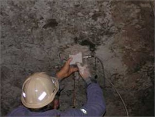
A rigid connection between sensor and rock is ensured, since the sensor is mounted using gypsum binder. Primarily, the sensor was located 20 m from the mining face and the distance was increasing up to 140 m, due to advance of mining works. In this paper we analyze 2 exemplary signals with sources located approx. 110-130 m from the sensor.

3. Methodology

Seismic signals are known to be non-stationary, since e.g. their amplitude spectra are time-varying during the entire record. Thus, we analyze seismic signals by fitting a sliding-window AR model, which is basically a set of AR models fitted to a consecutive, overlapping windows. The classical zero-mean autoregressive model of order $p$ is defined as [14]:

where ${\varphi }_1$,…, ${\varphi }_p$ are the autoregression parameters and ${\epsilon }_t$ is white noise. Recall, that the order of AR model might be related to the frequency structure (amplitude spectrum) of the considered signal. To wit, complex roots of the characteristic polynomial are related to local maxima of the signal‘s amplitude spectrum. Thus, if the amplitude spectrum consists of $P/$2 significant local maxima, then the AR model order must be no less than $P$ in order to address every significant local maximum of the amplitude spectrum. The higher order – the better approximation of the amplitude spectrum. Another parameter of the sliding-window AR model is length of the window. In this study we use 60-sample long Hamming window, which corresponds to 48 ms of the recording and AR model order is set to 10. Each pair of consecutive windows share 59 samples of the signal, thus every change of considered characteristics is manifested. A discussion on other lengths of the window and other orders of AR model is contained in section 4. The AR model is fitted to each window using Yule-Walker equations [14]. Then, amplitude, phase and group delay responses of each AR model are considered. Such analysis give information about volatility of these properties of the signal. In this paper we focus on group delay due to its interpretation and ability to distinguish two signals with similar time series and amplitude responses of the sliding-window AR model. Group delay is defined as a negative derivative of the phase with respect to frequency:

We refer to [15], where the numerical algorithm for computing the group delay of an IIR filter is explained. In this study we analyze group delay map of sliding window AR model, which represents group delay from AR model fitted to each window.

In the literature one can find several interpretations of group delay related to time required for a pulse to traverse a given displacement [16] or speed of energy transport through the system [17]. The explanation of group delay related to the propagation time of impulse response of the linear filter [18] is the most appropriate in this case. According to this interpretation, the group delay provides information regarding with what delay the frequency components of the signal are passed from the source to the sensor. Therefore, significant variations of group delay might reveal significant changes in signal propagation.

4. Real data results

Fig. 2 and Fig. 3 show two signals (4_45 and 4_48) representing vibration acceleration acquired by the sensor in two different days. Each of the signals has similar time series – the amplitudes suddenly gain and decay to the level of seismic noise.

Fig. 2Signal 4_45: a) time series and time-frequency maps of b) amplitude, c) phase and d) group delay response of sliding-window AR model

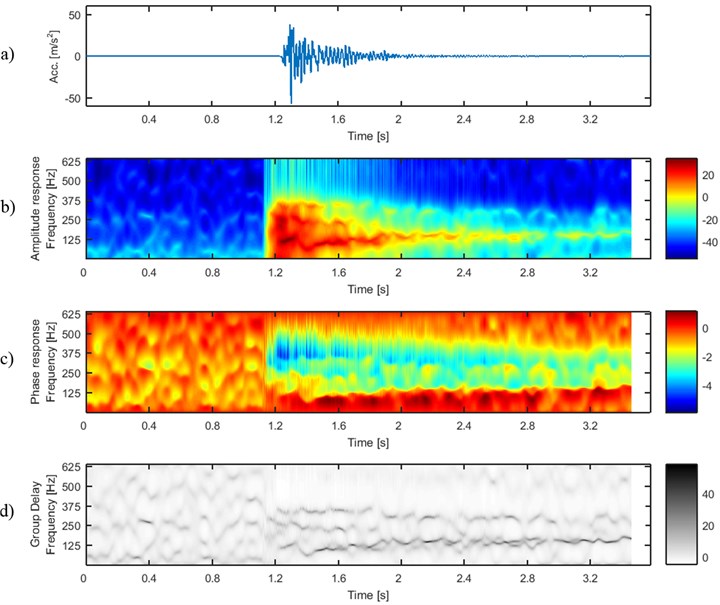
Time-frequency maps representing the AR model‘s amplitude response (ARgram) are also similar. In each case at the beginning of the signal the amplitude response has low values (seismic noise), but when the window begins to include samples with higher acceleration, one can perceive a sudden increase of amplitude response. Most of the signal’s energy is contained in frequency band close to 125 Hz and 250 Hz. However, the highest values of amplitude can be noticed at the frequency band close to 125 Hz and energy contained therein remains until the amplitude of the signal reaches the level of seismic noise. Other frequency bands are damping much faster.

Fig. 3Signal 4_48: a) time series and time-frequency maps of b) amplitude, c) phase and d) group delay response of sliding-window AR model

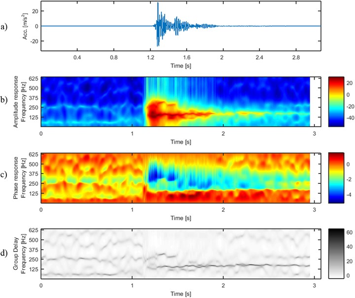
It is a really challenging problem to distinguish between these two signals taking into account shape of time series or amplitude response of sliding-window AR model. One can notice that phase responses are slightly different, i.e. ratio between phase response at 125-250 Hz (black frame) and at 250-500 Hz (white frame) is different for both of the signals. To wit, in 4_45 the phase is close to –2 at 125-250 Hz (yellow color) and close to –4 at 250-500 Hz (blue color), but in 4_48 the phase is close to –4 in both bands. Although, the difference is rather small and difficult to quantify, since in every frame the dominating phase is contaminated by areas with phases different to –2 or –4. The solution to this problem is provided by group delay responses of sliding-window AR models (Fig. 2(d), Fig. 3(d)). One can easily notice that before the P-waves arrive, the group delays are similarly scattered in both of the signals and time-frequency maps are blurred therein. Then, 3 ridges of group delay arise in 4_45 at frequencies approx. 125, 250 and 375 Hz. At about $t=$0.75 s the two latter ridges drop off and just one remains, at 300 Hz. In 4_48 two ridges (approx. 125 and 300 Hz) arise when P-wave arrives. At $t=$0.5 the latter ridge suddenly disappears and the ridge at 125 Hz remains only. Contrary to the amplitudes of the signals (including amplitudes at particular frequency bands), values of group delay at mentioned frequencies are not damping – similar level of group delay is evident up to the end of signal duration.

The analysis is performed using a fixed 60-sample long window and AR model order equal to 10. The AR model order is strictly related to the number of dominating spectral components and higher order approximates the impulse response of the model better than lower AR model order. Thus, one can expect better resolution at a given time point using higher order of AR model. In time-frequency analysis, the window length is responsible for better time or frequency resolution. Thus, one can expect a more smooth transition of three ridges into two ridges in Fig. 2(d) with a longer window. Although, the key properties that distinguish between two group delay time-frequency maps are obtained for the same set of sliding-window AR model parameters, i.e. window length 60 and AR model order 10. Therefore, similar difference between group delays for these two signals are expected for slightly different set of these parameters.

5. Conclusions

In this paper the group delay time-frequency map is presented as a tool for distinguishing between two similar seismic signals. These signals are similar in terms of time series and amplitude responses of sliding-window AR model. Contrary, the patterns at the group delay time-frequency map are different for each signal. Due to the physical interpretation of group delay, the possible reason that caused difference in group delay maps is related to sudden change of the system in terms of wave propagation. The discussion on different parameters of the sliding-window AR model promises robustness of the result on different length of the window and AR model order. Future work on the group delay time-frequency representation might be related to quantification of the differences in a relatively small set of parameters. Of course, size of the set of parameters should be equal for signals with different duration – it will make possible to group the signals using a clustering method. Another application of the presented results might be related to segmentation of seismic signals, including picking the beginning of a seismic signal in noisy conditions.