Abstract
Due to the complexity of the crustal medium and stratigraphic boundaries, seismic waves typically exhibit attenuation and dispersion after propagation through the medium. By studying the regularity of seismic wave dispersion, soil layer information can be extracted. Current spectral decomposition techniques take less account of signal filtering processing of seismic waves, and the complexity of the stratigraphy tends to reduce the accuracy of dispersion analysis. Based on the above, a new method for calculating the dispersion characteristics of a site from surface and downhole ground vibration recordings is proposed, which is simpler than the spectra analysis of surface waves (SASW) method and eliminates the need for multiple pickups and additional equipment. This method is based on wavelet decomposition and seismic wave filtering, and a numerical simulation example is established to verify the effectiveness of the method. Then, the records of the Tohoku earthquake on March 11, 2011 are used as actual strong earthquake examples for filtering and dispersion analysis. Finally, it is concluded that the seismic wave dispersion analysis method based on wavelet decomposition can effectively filter and analyze seismic waves in specific frequency bands.
Highlights
- A seismic wave filtering method based on the energy point of view is proposed.
- The feasibility and accuracy of the method are verified by establishing a numerical simulation model.
- Seismic wave data in the north-south and east-west directions is used for dispersion characteristics study, respectively.
- The filtering and signal smoothing methods based on the energy perspective provides a potential new approach for frequency dispersion research.
1. Introduction
Wave propagation is characterized by the phenomenon of dispersion, which can be interpreted as a change in the waveform in space due to the different phase velocities of the components of the wave, resulting in a change in the energy distribution. The complexity of the crustal medium, stratigraphic boundaries, and the usual presence of rock pore structures containing fluids in the subsurface lead to complex attenuation and dispersion patterns of seismic waves [1]. Besides, strong ground motions generated by massive earthquakes can cause the Earth’s near-surface to soften and even lead to liquefaction in extreme cases. These changes may lead to a decrease in shear modulus and an increase in viscous damping [2]. The complex nonlinear characteristics of geotechnical materials under seismic action further exacerbate the attenuation and dispersion phenomena of seismic waves [3]. By studying the regularity of seismic wave dispersion, the information of underground medium carried in seismic waves can be extracted. Therefore, it is necessary to study the dispersion of seismic waves. Dispersion attribute studies of seismic waves require seismic data in different frequency bands, and hence time-frequency analysis of seismic data is required to obtain different frequency components [4]. Many methods can realize the spectral decomposition, such as Short Time Fourier Transform (STFT), Wavelet Transform (WT), S-transform, and Wigner-Ville distribution [5]-[6]. At present, the dispersion properties of seismic waves are usually studied without signal filtering during the time-frequency analysis process, and thus the attenuation and dispersion patterns of seismic waves are often difficult to be accurately identified due to the complexity of the stratigraphic structure. Based on the above, this paper proposes a wavelet decomposition-based wave velocity estimation and seismic wave filtering method, and establishes a numerical simulation example to verify the effectiveness. Then, the seismic records of the Tohoku Earthquake are used as the actual strong earthquake examples for filtering and dispersion analysis. Finally, it is concluded that the seismic waveform dispersion analysis method based on wavelet decomposition can effectively filter seismic waves and analyze the dispersion in a specific frequency band.
2. Wave velocity estimation and seismic wave filtering
2.1. Wave velocity estimation method
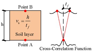
First, the Fourier spectra of the input and output signals are calculated separately and the coherence function is computed. Then the coherence function is zeroed out for any value that is too small (less than 0.01 times the maximum value). Afterwards, the inverse Fourier transform is performed on the frequency domain coherence function to obtain the coherence coefficient curve in the time domain. Then the estimation of shear wave velocity can be obtained from the following equation:
where is the thickness of the soil layer, and is the time length corresponding to the first peak in the coherence function curve that is greater than or equal to (shown in the Fig. 3). is the lower bound of the peak point of the coherence function, and is the upper bound of the shear wave velocity.
2.2. Wavelet decomposition-based filtering method
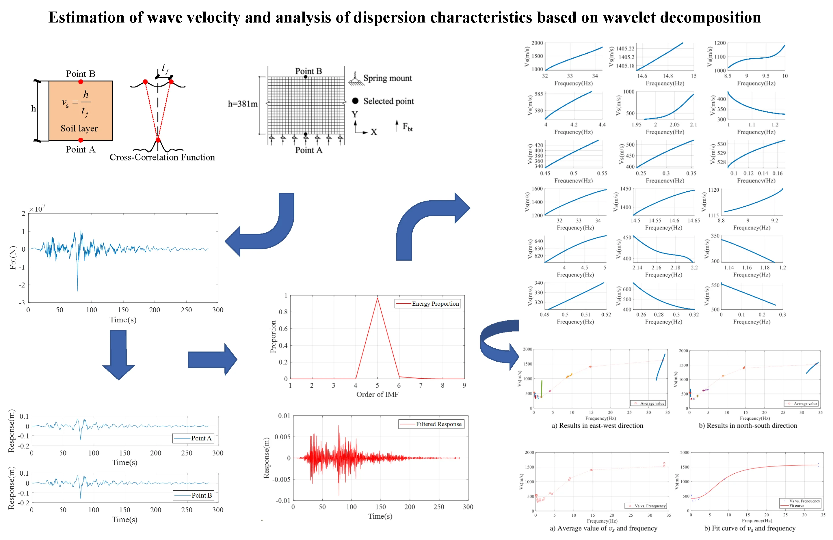
In this paper, utilizing wavelet decomposition as a means of signal processing, a seismic wave filtering method based on the energy point of view is proposed (shown in Fig. 1).
Fig. 1Flowchart of the method
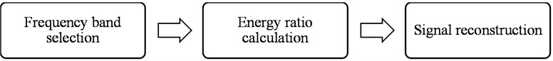
Before signal decomposition, it is necessary to determine a more appropriate frequency range, in which the signal energy needs to account for more than 90 % of the total energy. The determination of the frequency range needs to take into account the characteristic period of the seismic site, which needs to be set near the natural frequency. Due to the complexity of the stratigraphic structure, the seismic wave signals are usually very non-stationary. Therefore, focusing the frequency range of signal decomposition to the vicinity of the intrinsic frequency of the site can improve the accuracy of seismic wave dispersion analysis. The seismic waves are then decomposed into a total of intrinsic mode functions (IMFs) in the selected frequency band using wavelet decomposition. The energy of each IMF is then calculated as follows:
where denotes the Fourier transform of the th IMF, represents time, and denotes the total number of data points. Then the energy share of each IMF obtained from the seismic wave decomposition can be calculated. And then the representativeness of the signal components relative to the original seismic wave can be determined. Finally, the signal components with energy share less than 0.1 are filtered and the remaining IMFs are combined into a new seismic wave signal. Through the above filtering process, the low-energy clutter components in the frequency band can be eliminated.
3. Numerical modeling example
The feasibility and accuracy of the method are verified by establishing a numerical simulation model using SAP2000 software. Filtering and wave velocity calculations are carried out by using the data from the Tohoku Earthquake. A remote boundary homogeneous soil layer with a thickness of 381 m is modeled with the parameter settings shown in Table 1. The theoretical value of shear wave velocity for this layer is calculated using the following:
where represents the shear modulus and represents the density of the soil layer. The remote boundary homogeneous soil model has a spring support at the bottom of the model, which can simulate the input of seismic waves by inputting shear force and forward pressure (shown in Fig. 2). The distance between the left and right boundaries of the model is very far. When the seismic wave at the bottom has already traveled to the top, the seismic wave propagating to the left and right sides has not yet reached the boundary, which circumvents the influence of the reflection of seismic wave at the boundary of the two sides of the soil layer.
Table 1Soil parameters of numerical model
Parameter | Value |
Modulus of elasticity | 1.323×10¹⁰ Pa |
Shear modulus | 5.292×10⁹ Pa |
Density ρ | 2.7×10³ kg/m3 |
Poisson’s ratio | 0.25 |
Theoretical value | 1.400×10³ m/s |
Fig. 2Numerical model of soil layers
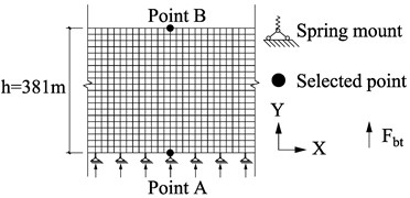
Fig. 3Schematic diagram of the vs calculation
Firstly, the shear force which will be applied to the spring mount of the model is calculated based on the seismic wave record shown in Eq. (4), where is the spring stiffness coefficient on the viscoelastic boundary, is the spring damping coefficient on the viscoelastic boundary, is the incident wave displacement, is the incident wave velocity, and is the shear wave velocity. The calculation of coefficients and is shown in Eq. (5), where is the viscoelastic boundary correction factor, taken as 0.5, is the shear wave velocity of the soil layer, represents the density of the soil layer (shown in Table 1), and is the distance from the wave source to the artificial boundary:
Then the (as the ground excitation) is input to the bottom boundary of the soil layer for simulation, and the time curve data of point A (mid-point at the bottom) and point B (mid-point at the top) is extracted after the simulation. Using the method of Sections 2.1 -2.2, the estimated shear wave velocity of this formation can be calculated and finally compared with the theoretical value to verify the accuracy of the method.
Fig. 4Time history of Fbt
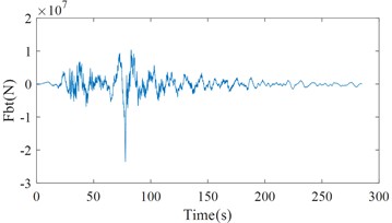
Fig. 5Numerical simulation results of point A and B
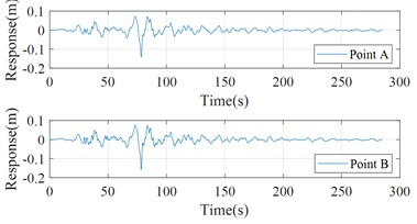
The seismic records from the KiK-net station in Japan for the Tohoku earthquake are selected for calculation. Taking the seismic wave record MYGH041103111446NS1 as an example, the shear force applied to the spring at the bottom of the model by the simulated seismic wave input is first calculated (shown in Fig. 4). The seismic response curves at the bottom midpoint and top midpoint of this soil model are shown in Fig. 5.
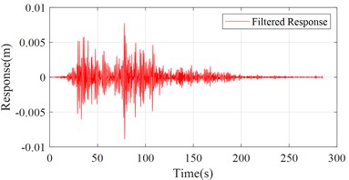
From the aforementioned parameters of the soil model, the characteristic period of the soil layer can be calculated to be about 1.088 s, and the intrinsic frequency is about 0.919 Hz. The initial frequency band is [0.5, 2.0] Hz interval, and it is calculated that the energy of the signal in the band accounts for 99.92 % of the total energy, which meets the requirements. Then the displacement response of point B is decomposed by wavelet decomposition and the energy share of each IMF is calculated in the frequency band of [0.5, 2.0] Hz interval (shown in Fig. 6). From this, the IMF components with an energy share greater than 0.1 can be selected and the signal reconstruction is performed to obtain the new response of point B (shown in Fig. 7). It can be seen that the spurious components in the response time history of the simulation model are removed. The response of point A and filtered response of point B will be used as the input and output respectively to calculate the shear wave velocity . The calculated estimation value of is 1.465×10³ m/s, which is close to the theoretical shear wave velocity of 1.400×10³ m/s.
Fig. 6Energy proportion of IMFs
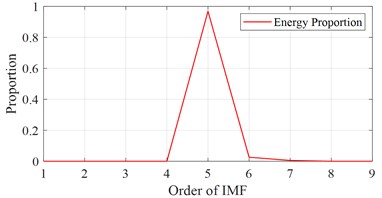
Fig. 7Filtered response of point B
4. Dispersion analysis of seismic waves
Still using the records MYGH04 of the Tohoku earthquake as an example for processing and analysis. Seismic wave data in the north-south and east-west directions is used for dispersion characteristics study, respectively. Firstly, considering the complexity of the stratigraphy and the fact that soil movement due to seismic action can have an impact on the propagation of seismic waves, it is necessary to pre-process records from surface station. In order to reduce the errors of the station's sensors under strong seismic effects, the first 15 s of seismic data are removed. Then the seismic wave data from surface are decomposed into multiple intrinsic mode functions (IMFs) based on wavelet decomposition. Using the estimation method of in Section 2.1, each IMF component can be processed to obtain the corresponding time-varying . The relationship between shear wave velocity and instantaneous frequency is then obtained by using the Hilbert transform to obtain the frequency corresponding to each time point. The relationship between shear wave speed and instantaneous frequency is then obtained by using the Hilbert transform to obtain the frequency corresponding to each time point. However, the relationship curve directly calculated by the above process has many spikes and clutter components, so it needs to be further filtered to make the result smooth. Filtered results are shown in Figs. 8-9.
Fig. 8Wave velocity vs and frequency in east-west direction of IMFs
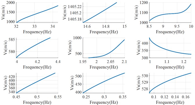
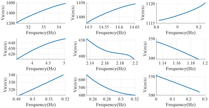
Fig. 9Wave velocity vs and frequency in north-south direction of IMFs
The and instantaneous frequency calculated from each IMF are then processed to obtain the average values based on empirical modal decomposition (EMD) method. In short, based on EMD, the and instantaneous frequency calculated from each IMF can be decomposed into multiple signal components again separately. The energy share of the newly decomposed signal components is used as a weighting factor to calculate the weighted average value of and instantaneous frequency corresponding to each of the original IMFs, respectively. The results are shown in Fig. 10. Once the data from MYGH04 in the north-south and east-west directions have been calculated, the results in both directions can be combined to obtain dispersion results for the site (shown in Fig. 11(a)). A smoother result can be obtained after fitting the results of average value (shown in Fig. 11(b)). The mathematical expression used to fit the curve is as follows:
where represents the fitted value of, and represents instantaneous frequency. Besides, 424.5, 2.727, 8.027, 1596. It can be seen that the estimated at the site increases with increasing instantaneous frequency in the [0, 20] Hz band. And after the 20 Hz band, the will grow in a slower trend and gradually stabilize.
Fig. 10Weighted average values of vs and frequency from IMFs
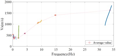
a) Results in east-west direction
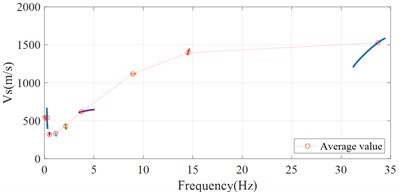
b) Results in north-south direction
Fig. 11Dispersion analysis results of the site MYGH04
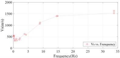
a) Average value of and frequency
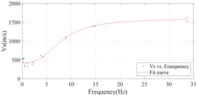
b) Fit curve of and frequency
5. Conclusions
In this paper, a wavelet decomposition-based wave velocity estimation and seismic wave filtering method is proposed, and the seismic records of the Tohoku Earthquake are used as the actual strong earthquake examples for dispersion analysis. Based on numerical simulation results and the analysis results of seismic record MYGHO4, the following conclusions are drawn.
1) This wave velocity estimation method can accurately calculate the of site.
2) The wavelet decomposition-based seismic wave filtering method can effectively preprocess seismic wave data, filtering out low-energy clutter components through signal decomposition and reconstruction.
3) The filtering and signal smoothing methods based on the energy perspective can effectively overcome the difficulties caused by the complexity of soil layer structure in analysis, providing a potential new approach for frequency dispersion research.
References
-
W. Shen et al., “A seismic reference model for the crust and uppermost mantle beneath China from surface wave dispersion,” Geophysical Journal International, Vol. 206, No. 2, pp. 954–979, Aug. 2016, https://doi.org/10.1093/gji/ggw175
-
K. van Wijk and A. L. Levshin, “Surface wave dispersion from small vertical scatterers,” Geophysical Research Letters, Vol. 31, No. 20, Oct. 2004, https://doi.org/10.1029/2004gl021007
-
Y. Wang, S. Chen, L. Wang, and X.-Y. Li, “Modeling and analysis of seismic wave dispersion based on the rock physics model,” Journal of Geophysics and Engineering, Vol. 10, No. 5, Oct. 2013, https://doi.org/10.1088/1742-2132/10/5/054001
-
Y. Chen, “Nonstationary local time-frequency transform,” Geophysics, Vol. 86, No. 3, pp. V245–V254, May 2021, https://doi.org/10.1190/geo2020-0298.1
-
J.-C. Hong, K. H. Sun, and Y. Y. Kim, “Dispersion-based short-time Fourier transform applied to dispersive wave analysis,” The Journal of the Acoustical Society of America, Vol. 117, No. 5, pp. 2949–2960, May 2005, https://doi.org/10.1121/1.1893265
-
L. Jiang, W. Shang, Y. Jiao, and S. Xiang, “An Adaptive Generalized S-Transform Algorithm for Seismic Signal Analysis,” IEEE Access, Vol. 10, pp. 127863–127870, 2022, https://doi.org/10.1109/access.2022.3227426
About this article

The authors have not disclosed any funding.
The datasets generated during and/or analyzed during the current study are available from the corresponding author on reasonable request.
The authors declare that they have no conflict of interest.
