New approaches to pattern discovery in signals via empirical mode decomposition

1.1. IMF classification

Although much work on EMD and its applications to different signals has already been done [1, 3], a general classification for different kinds of obtained IMFs has not been introduced yet. Therefore, we would like to draw attention to this problem because not only does it have theoretical significance, but it also gives an opportunity to develop more effective techniques in order to cope with many problems of signal processing (pattern discovery, denoising, etc.). All IMFs may be divided into two big groups:

• Significant IMFs – including noise-like IMFs and IMF-patterns;

• Trend-like IMFs – including true trend-like IMFs and compensating (spurious) IMFs.

Significant IMFs always have an exact origin (their appearance may be explained using the observed signal) and characterize signal’s internal structure and features inherent of a signal. According to the suggested classification, significant IMFs comprise noise-like IMFs and IMF-patterns. The former is caused exclusively by unwanted and contaminating noise in the original signal. Such IMFs are frequently dealt with since noise’s presence is almost inevitable in practice. This group of IMFs usually consists of several components each approximating noise with different accuracy. Due to a wide spectrum and oscillating nature, noise-like IMFs are found at initial decomposition levels, as follows from the dyadic filter bank structure [1]. It is quite obvious that such components are undesirable; nevertheless, their origin may be established and they may usually be identified. IMF-patterns, on the contrary, represent components connected with a useful (wanted) signal and their extraction is one of the main objects of EMD. These patterns often contain unique distinguishing information about the given signal and make this signal different from other similar ones.

Trend-like IMFs always complete decomposition and have the lowest average frequencies among the extracted IMFs. They belong to a separate category of components because very often they have no physical interpretation or direct relation to the original signal, unlike the significant IMFs introduced above. If a signal has the mean trend, this trend may be extracted after analyzing such IMF types. For example, if we simulate a pure monoharmonic signal added to a slowly varying polynomial (the degree range being 3-5) and subject this mixture to EMD, we will obtain true trend-like IMFs approximating this polynomial.

Spurious trend-like IMFs, which may be also called compensating IMFs, are a result of EMD’s shortcomings and arise only for this reason. There are several main modifications of EMD [1], all of which may turn out to be responsible for such IMFs. The main reasons for their appearance are some negative effects of cubic spline interpolation (end effects, undershoots, overshoots), calculation errors, and inappropriate sifting criteria. Such IMFs must be removed because they do not usually carry any substantial information about a signal. What is more, they cause redundancy and may consume additional memory resources during computer processing. The name “compensating” implies that their sum is close to zero, therefore, they virtually compensate each other. In order to avoid them and prevent the distortion of the whole decomposition some preprocessing ought to be carried out. There are special techniques for suppressing large end oscillations – mirroring extrema, zero-padding, signal extension, etc. The sifting criterion should be selected very carefully. Also, it is possible to use other ways of interpolating extrema or construct one envelope connecting all maxima and minima instead of two separate ones.

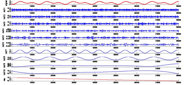
The example in Fig. 1 elucidates the new notions (IMF types) introduced for the purpose of understanding EMD’s performance in greater depth. The vibrational signal is a biharmonic one consisting of two monoharmonics with equal unit amplitudes and frequencies differing by a factor of 2. This frequency ratio has been chosen with the view of revealing the EMD’s dyadic filter bank structure. In the remainder of the paper we will assume that signals are embedded in additive noise which follows Gaussian distribution with mean zero and some standard deviation (here standard deviation is 0.1).

After running EMD 10 IMFs and the final residual are obtained. The first six IMFs are noise-like. IMFs 7 and 8 in Fig. 1 are the corresponding monoharmonics appearing in frequency-descending order. These two monoharmonics are IMF-patterns since they contain information about the pure original signal. Finally, the last three components are compensating ones, their sum being very close to zero. They are meaningless since they do not provide any information about the signal but only cause redundancy.

The proposed classification of IMFs is not only an attempt to replenish the insufficient amount of the existing EMD theory but also a powerful and reliable means of solving some very important practical goals: 1) Removing noise (denoising); 2) Discovering typical patterns; 3) Eliminating compensating IMFs and avoiding redundancy.

Fig. 1EMD of a biharmonic signal (the signal is plotted first)

The problem of denoising has been addressed in a number of publications and several techniques have been tested. For example, EMD-thresholding, which acts to remove noise by analyzing IMF samples independently and either setting to zero those that are small in magnitude (hard-thresholding) or reducing the magnitudes of some samples attributed to noise, which we wish to remove (soft-thresholding). Furthermore, there is an energy estimation approach [1]. All of them require initial parameters which are often difficult to select accurately. Here we propose new methods based on the classification above, special criteria and numerical identification of noise-like components. They are mostly devoid of any tuning, work automatically and may be deduced rigorously. So far, a wide range of pattern discovery techniques has been introduced [1, 3], but the vast majority of them are too specific and provide adequate results only in particular knowledge domains making it difficult for experts in other fields to adapt all these methods. Concerning redundant IMF removal, it has been addressed in [3] with an idea of parabolic (instead of spline) envelope interpolation and specifying the location of extrema. However, this method might prevent them from arising but it does not guarantee that they will not appear, in which case it will be necessary to recognize and remove them. Thus, in an attempt to offer a more effective and flexible solution of all these problems simultaneously we will try new methods based on the classification offered and the criteria covered in the previous section.

1.2. Regression-based IMF classification

In this section, we are going to offer an approach to pattern discovery partly borrowed from the regression theory and providing an opportunity of numerical identification of various kinds of IMF. Hence, it will be possible to determine the IMF’s type by means of a statistic specially designed for this purpose. This approach seems the most promising for further investigation among all the ones expounded in the present paper since it possesses the highest classification accuracy and may be deduced rigorously from some basic equations of EMD and statistics.

The procedure begins by representing a signal’s model in the way corresponding to the standard classical regression problem:

where $s$ denotes the vector containing samples of the original signal, $x$ is a matrix of regressors, $\beta$ is a vector of unknown coefficients, each specifying the weight of a particular regressor, $e$ is white Gaussian noise $N(0;{\sigma }^2)$.

Consider the connection between the extracted IMFs and the observed signal (originally introduced in [1]):

The first term may be regarded as an approximation of the original noise since it has the largest average frequency and is most strongly affected by noise. Under this assumption, we arrive at:

Now one more specification is required. It is known that EMD’s convergence has yet not been proven rigorously apart from some particular cases, which cannot be generalized. Even though the convergence problem, in a strict mathematical sense, is acknowledged to be one of the drawbacks of EMD, it is still possible to elaborate EMD and slightly reduce this problem. In view of these facts, convergence is usually understood in engineering sense, i.e. the maximum absolute difference between the original signal and the sum of all extracted components is a very small quantity, often indistinguishable from zero. Hence, one sensible approach to this problem is to introduce special coefficients for each IMF, which are calculated via the least-squares method. These weight coefficients aim at improving the accuracy of signal reconstruction:

where $\beta$ is a vector of coefficients to be discovered. The equation above may take a more familiar vector-matrix form:

where $C$ is a matrix whose columns store IMF samples (the number of columns is less by one than the number of components obtained after EMD because the first IMF, being noise approximation, is not included in this matrix). The least-squares estimate of vector $\beta$ is reduced to:

For model coefficients, it is possible to provide an interval estimate, i.e. to find the boundaries to which a particular regression coefficient is delimited with the given confidence probability $P$ (in our example, $P=$ 0.95). The boundaries of the confidence interval ($CI$) are defined as:

where ${\beta }_i$, ${\tilde{\beta }}_i$ are the true value of $i$th regression coefficient and its estimate, respectively, and $t_{\gamma }$ is a fractile of $t$-distribution.

The next and final step is the most significant. All coefficients may be subjected to a statistical significance test as is often done in the classical regression problem:

where $V$ is a covariance matrix of IMFs calculated as $V=C{C}^T$, ${\tilde{\sigma }}_e$ is an estimate of standard deviation of noise. It is necessary to consider two alternative hypotheses. One of them states that a coefficient is equal to zero (is statistically insignificant) – null hypothesis $H_0$, whereas the other one states the opposite (nonnull hypothesis $H_1$). Significance may be tested by the statistics given above, which has t-distribution if hypothesis $H_0$ is valid. However, in our case all coefficients are apriori significant because all components are included in signal reconstruction with non-zero weight coefficients. Thus, the null hypothesis is rejected. However, the results obtained after calculating Eq. (10) (Table 1) suggest that this statistic may be regarded as a classification statistics, assigning IMFs to one of the three groups and allowing us to achieve the aims of discovering patterns, denoising and eliminating spurious IMFs. In order to find a suitable estimate ${\widehat{\sigma }}_e$ for Eq. (10) it is possible to employ the one originally proposed in wavelet context and known as median absolute deviation (MAD):

The MAD estimator is robust against large deviations and should therefore reflect noise standard deviation (s.d.). The results of calculations for the multiharmonic signal (in Fig. 1) are given in Table 1.

Judging from the results for $T_1$, as seen in Table 1, an important conclusion may be drawn: the values of the statistics are significantly different for various IMF types – for IMF-patterns and all the rest (noise-like and trend-like) ones. On the basis of the values (shown in bold in Table 1) obtained for the 6th, 7th and 8th IMFs (which correspond to pure monoharmonics in the vibrational signal) we may declare that they belong to IMF-patterns, while all the rest are either noise-like or trend-like IMFs. Cluster-analysis [4] performs this classification automatically, which is another advantage of the whole method. For instance, the well-known $k$-means and EM algorithms are quite suitable here with the number of clusters equal to 2. In the end, two groups (clusters) will be found to accord with IMF types. In some cases, for a more detailed classification, the number of clusters may be set at 3 in order to obtain three separate clusters containing IMF-patterns, noise-like IMFs and trend-like IMFs, respectively. The column containing CI lengths in Table 1 also requires attention since CI lengths are different for the considered types of IMFs. These lengths do not depend on a particular value of any coefficient see Eq. (9) and they are the smallest for IMF-patterns (equal to 0.002). Thus, this parameter may also be an attribute in the classification procedure.

References

-
Huang N. E., Shen S. S. P. The Hilbert Transform and its Applications. World Scientific, 2005.
Stoica P., Moses R. Spectral Analysis of Signals. Upper Saddle River, New Jersey, 2005.
Rato R. T., et al. On the HHT, its problems, and some solutions. Mechanical Systems and Signal Processing, 2007.
Witte I. H., et al. Data Mining: Practical Machine Learning Tools and Techniques with Java Implementation. Academic Press, 2000.
About this article
The paper is supported by the Contract No. 02.G25.31.0149 dated 01.12.2015 (Ministry of Education and Science of the Russian Federation).