State-space approach to 3D generalized thermoviscoelasticity under Green and Naghdi theory II

1. Introduction

In 1967, Lord and Shulman [1] established a mathematical model of generalized thermoelasticity which referred as ‘LS model’ in order to eliminate the paradox of infinite speed of propagation of thermal disturbances [2]. In LS theory the classical Fourier’s heat conduction equation has been modified by introducing a parameter called relaxation time and the heat conduction equation becomes hyperbolic in nature and thus finite speed of propagation of heat pulses is predicted. After five years of LS theory, Green and Lindsay [3] formulated another model (referred as ‘GL model’). In this model, the Fourier’s law of heat conduction remains unchanged whereas the classical energy equation and the constitutive equation were modified by introducing temperature-rate-dependent terms. In GL model, two relaxation time parameters have been introduced. This model is often called as temperature-rate-dependent thermoelasticity (TRDTE).

Green and Nagdhi [4-6] proposed three theories of generalized thermoelasticity. The first model (GN I) is exactly the same as Biot’s theory [2]. The second and third model is labeled as GN II and GN III model. In GN II and GN III models, the thermal wave propagates at finite speed. An important feature of GN II model is that this model does not accommodates dissipation of thermal energy whereas GN III model accommodates dissipation of energy. One can see the publications [7-15] for many investigations using GN II model. The theoretical investigation and application in thermoviscoelastic materials have become a significant task for solid mechanics due to the rapid development of polymer science and plastic industry as well as the wide use of materials under high temperature in modern technology. Keeping this fact in mind, many researchers [16-25] studied several problems on wave propagation in linear thermoviscoelastic and electro-magneto-thermoviscoelastic solid.

In the present paper, our main goal is to apply the state-space approach to study the effects of viscosity on a three-dimensional thermoelastic homogeneous isotropic half-space solid body whose surface is subjected to a thermal shock and is assumed to be stress free. The formulation is applied to the generalized thermoelasticity based on the GN model without energy dissipation. The normal mode analysis [9, 26] together with state-space approach [27-30] is used to obtain the exact analytical expressions for the variables considered. Numerical computations are performed for a specific material and the results obtained are represented graphically. Comparisons are made within the theory in the presence and absence of viscosity effects.

2. Governing equations

Following [5], the strain-displacement relations, the stress-strain-temperature relations, the equations of motion in absence of body forces and the heat conduction equation in absence of heat source for a homogeneous isotropic thermally conducting viscoelastic solid may be written as:

where:

where $e_{ij}$ are the components of strain tensor, ${\sigma }_{ij}$ are the components of the stress tensor, $\lambda$, $\mu$ are Lame’s constants, $\gamma =(3\lambda +2\mu ){\alpha }_T$ is a material constant characteristic of the theory, ${\alpha }_T$ is the coefficient of linear thermal expansion, $\rho$ is the density, ${\delta }_{ij}$ is Kronecker delta, $u_i$are the components of the displacement vector, $k^{\mathrm{*}}\mathrm{}(>0)$ is a material constant characteristic of the theory, $C_E$ is the specific heat at constant strain, $T$ is the temperature change, $T_0$ is the reference temperature of the medium assumed to be such that $|T/T_0|\ll \text{1}$, $e=e_{kk}$ is the cubical dilatation, ${\lambda }_0$, ${\mu }_0$, ${\gamma }_0$ are viscoelastic constants and ${\nabla }^2\equiv {\partial }^2/\partial x^2+{\partial }^2/\partial y^2+{\partial }^2/\partial z^2$.

3. Formulation of the problem

We shall consider a homogenous isotropic thermoviscoelastic solid medium in three-dimensional space which fills the region:

and is subjected to a time dependent heat source on the bounding plane to the surface $x=0$. Moreover, the body is initially at rest and the surface $x=0$ is assumed to be stress free. The initial conditions on all the physical variables are taken to be homogeneous. We shall use the cartesian coordinates $\left(x,y,z\right)$. The displacement components thus have the form $u_i=\left(u,v,w\right)$. Hence the governing equations take the following form:

where:

and a subscript comma denotes spatial derivatives and a superimposed dot represents differentiation with respect to time.

In order to non-dimensionalize the above equations, we define the following non-dimensional parameters:

where $l$ is some standard length.

Introducing the above non-dimensional parameters in Eqs. (5)-(14) and using the relation Eq. (15), we obtain the following set of governing equations (suppressing the primes for convenience):

where $\epsilon ={\gamma }_e^2{T}_0/\left[\rho C_E\left({\lambda }_e+2{\mu }_e\right)\right]$ is the dimensionless thermoelastic coupling parameter, $C_T=c_3/c_1$ is the non-dimensional finite thermal wave speed of GN theory, $c_1=\sqrt{\left({\lambda }_e+2{\mu }_e\right)/\rho }$ is the longitudinal waves speed, $c_3=\sqrt{k^{\mathrm{*}}/\rho C_E}$ is the finite thermal waves speed of G-N theory and $\beta ={\mu }_e/({\lambda }_e+2{\mu }_e)$.

Taking differentiation of Eqs. (16), (17), (18) with respect to $x$, $y$, $z$ respectively and then adding we get:

We shall consider the invariant stress $\sigma$ to be the mean value of the principal stresses ${\sigma }_{ij}$ as follows [9]:

Adding the Eqs. (20)-(22) and using Eqs. (15) and (27) we get:

4. Normal mode analysis

The solution of the physical variables can be decomposed in terms of normal modes [9, 26] in the following form:

where $u^{\mathrm{*}}\left(x\right)$ etc. are the amplitude of the function $u(x,y,z,t)$ etc., $i$ is the imaginary unit, $\omega$ (complex) is the time constant and $a$, $b$ are the wave number in the $y$ and $z$ direction respectively.

Using (29) in the Eqs. (19), (26), (28) and then eliminating $e^{\mathrm{*}}\left(x\right)$ from the resulting equations we obtain:

where:

Choosing ${\theta }^{\mathrm{*}}$ and ${\sigma }^{\mathrm{*}}$ as state variables in the $x$-direction, Eqs. (30) and (31) can be written in a vector-matrix differential equation as follows:

where:

The initial conditions of the problem are assumed to be homogeneous and for the stress-free surface $x=$ 0, we assume the boundary conditions in non-dimensional form as follows:

(i) The thermal boundary condition is:

where $q_n$ denotes the normal component of the heat flux vector, $\nu$ is Biot’s number and $r(0,y,z,t)$ represents the intensity of the applied heat sources on $x=0.$

All the physical quantities are assumed to be bounded as $x\to +\mathrm{\infty }$. In order to use the above thermal boundary condition, we use the generalized Fourier’s law of heat conduction in the non-dimensional form, namely:

From Eqs. (33), (34) and (29) we obtain:

where $D=d/dx$.

(ii) Mechanical boundary condition that the bounding plane to the surface $x=0$ has no traction anywhere so we have:

which gives on using the normal modes Eq. (29):

5. State space approach

The formal solution of the vector-matrix differential Eq. (32) can be written as (see [27-30] for details):

where:

and we have used the boundary conditions Eq. (36) and the constant ${\theta }_0^{\mathrm{*}}$ is to be determined from the boundary conditions Eq. (35).

In the solution Eq. (37) we have omitted the positive exponential part to obtain a bounded solution for large $x$. Now, we shall first find the form of the matrix $\mathrm{e}\mathrm{x}\mathrm{p}\left[-\sqrt{A\left(\omega \right)}x\right]$.

The characteristic equation of the matrix $A\left(\omega \right)$ can be obtained as:

Let ${\lambda }_1$ and ${\lambda }_2$ be the roots (distinct) of the Eq. (39), where:

The spectral decomposition of the matrix $A\left(\omega \right)$ from [31] can be written as:

where $E$ and $F$ are called the projectors of $A\left(\omega \right)$ satisfying the following conditions (see [31] for details):

Now $\sqrt{A\left(\omega \right)}$ has the same projectors as of $A\left(\omega \right)$ (see [31]) and if $p_1$, $\mathrm{}{p}_2$ are the eigenvalues of $\sqrt{A\left(\omega \right)}$ then $p_1=\sqrt{{\lambda }_1}$, $p_2=\sqrt{{\lambda }_2}$. Hence the spectral decomposition of the matrix $\sqrt{A\left(\omega \right)}$ can be written as:

where:

and $E$, $F$ satisfy Eq. (41).

Thus, we find:

The Taylor series expansion of the matrix exponential in Eq. (37) has the form:

Using the Cayley-Hamilton theorem we can express ${A^{\mathrm{*}}}^2\left(\omega \right)$ and higher orders of the matrix $A^{\mathrm{*}}\left(\omega \right)$ in terms of $I$ and $A^{\mathrm{*}}\left(\omega \right)$, where $I$ is the second order unit matrix. Thus, the Taylor series in Eq. (45) can be reduced to:

where $a_0\left(x\right)$ and $a_1\left(x\right)$ are coefficients depending on $x$ only.

By Cayley-Hamilton theorem, the characteristic roots $p_1$ and $p_2$ of the matrix $A^{\mathrm{*}}\left(\omega \right)$ must satisfy Eq. (46) and thus we get:

The solution of the above system of Eqs. (47) and (48) is given by:

From Eqs. (46) and (49), we obtain:

where:

Finally, the solution of the vector-matrix differential Eq. (32) can be written in the form:

Hence using Eqs. (38), (51) and (52) in (53) the field variables ${\theta }^{\mathrm{*}}\left(x\right)$ and ${\sigma }^{\mathrm{*}}\left(x\right)$ can be obtained as:

where ${\theta }_1={\theta }_0^{\mathrm{*}}(C_1-{\lambda }_2)/\left({\lambda }_1-{\lambda }_2\right)$, ${\theta }_2={\theta }_0^{\mathrm{*}}(C_1-{\lambda }_1)/({\lambda }_1-{\lambda }_2).$

The boundary condition Eq. (35) gives the value of the constant ${\theta }_0^{\mathrm{*}}$ as:

By using Eqs. (29), (54) and (55) with Eq. (28) we get the cubical dilatational $e^{\mathrm{*}}\left(x\right)$ as:

where:

To get the displacement component $u^{\mathrm{*}}\left(x\right)$ we will use Eq. (16). By using Eqs. (29), (54) and (56) in the Eq. (16) we can write:

where:

The general solution of the ordinary differential Eq. (57) can be written as:

where ${\lambda }_1^2\ne {\lambda }_2^2\ne {\lambda }_u^2$ and $u_0$ is a constant to be determined from the boundary conditions Eq. (36).

Using Eqs. (29), (54), (56) and (58) in the Eq. (20) we obtain the stress components ${\sigma }_{xx}^{\mathrm{*}}\left(x\right)$ as:

where:

With the help of the boundary condition Eq. (36) and the Eq. (59) we obtain the constant $u_0$ as:

6. Numerical example and discussions

Since we have $\omega ={\omega }_0+i\zeta \text{,}$ where $i$ is the imaginary unit, $\mathrm{e}\mathrm{x}\mathrm{p}\left(\omega t\right)=\mathrm{e}\mathrm{x}\mathrm{p}\left({\omega }_{0}t\right)\left(\mathrm{c}\mathrm{o}\mathrm{s}\zeta t+i\mathrm{s}\mathrm{i}\mathrm{n}\zeta t\right)$ and for small values of time, we can take $\omega ={\omega }_0$ (real). For the discussions of the nature of dependence of all the physical variables on viscosity, we shall compute them numerically for a particular model. For this purpose, we choose the following numerical values of the relevant parameters for copper like material: (${\lambda }_e=$7.76×10¹⁰ N/m², ${\mu }_e=$3.86×10¹⁰ N/m², ${\lambda }_0=$0.06 s, ${\mu }_0=$ 0.09 s, ${\alpha }_T=$ 1.78×10^-5 K^-1, $C_E=$ 383.1 m²/K, $\rho =$8954 kg/m³, $T_0=$293 K, $\epsilon =$0.0168, $\beta =$ 0.25, $\omega =$3, $a=$ 1.2, $b=$ 1.3, $\nu =$50, $r^{*}=$ 100, $C_T=$2).

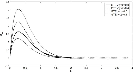
Using the above numerical values, the variations of the temperature distribution $\theta$, the mean stress $\sigma$, the displacement component $u$ and the stress component ${\sigma }_{xx}$ along $x$ axis at two different plane $y=z=\text{0.0}$ and $y=z=\text{0.4}$ for a particular time instant $t=\text{0.25}$ have been shown for (i) generalized thermoviscoelastic solid (GTVE) by solid line at $y=z=$ 0.0, $t=$ 0.25, (ii) generalized thermoviscoelastic solid (GTVE) by solid-dot line at $y=z=\mathrm{}$0.4, $t=\mathrm{}$0.25, (iii) generalized thermoelastic solid (GTE) by solid-dot (bold) line at $y=z=\mathrm{}$0.0, $t=\mathrm{}$0.25 and (iv) generalized thermoelastic solid (GTE) by dashed line at $y=z=\mathrm{}$0.4, $t=\mathrm{}$0.25. These variations are shown in Figs. 1-4.

Fig. 1Temperature distribution θ vs. x at t= 0.25

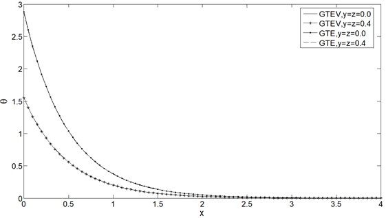
Fig. 2Mean stress distribution σ vs. x at t= 0.25

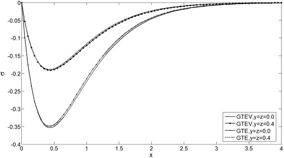
Fig. 3Displacement distribution u vs. x at t= 0.25

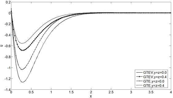
From Figs. 1-4 it is clear that $y$ and $z$ have decreasing effect on $\theta$, $\sigma$, $u$ and ${\sigma }_{xx}$ for both GTVE and GTE model for fixed $t$. Also it is depicted that the numerical values of $\sigma$, $u$ and ${\sigma }_{xx}$ are greater in GTVE model than GTE model for fixed $x$, $y$, $z$ and $t$ but Fig. 1 shows that the viscosity has no significant effect on $\theta$. The maximum value of all the physical quantities attain in the case of GTVE at the plane $y=z=\mathrm{}$0.0.

Fig. 4Stress distribution σxx vs. x at t= 0.25

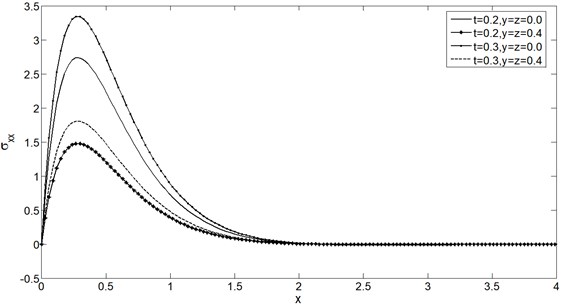
Figs. 5-8 show the distributions of $\theta$, $\sigma$, $u$ and ${\sigma }_{xx}$ for the GTVE model at $y=z=\mathrm{}$0.0 and $y=z=\mathrm{}$0.4 for two different time instants $t=\mathrm{}$0.2 and $t=$ 0.3. It is clear from all these figures that $t$ has increasing effects on all the physical quantities.

Fig. 5Temperature distribution θ vs. x for two time instants

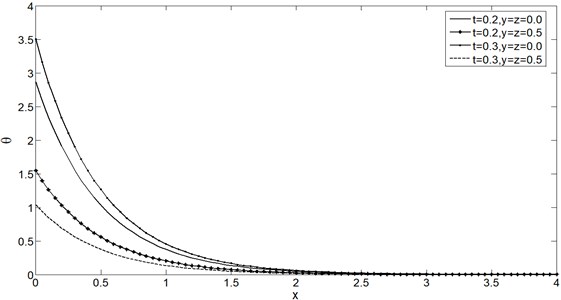
Fig. 6Mean stress distribution σ vs. x for two time instants

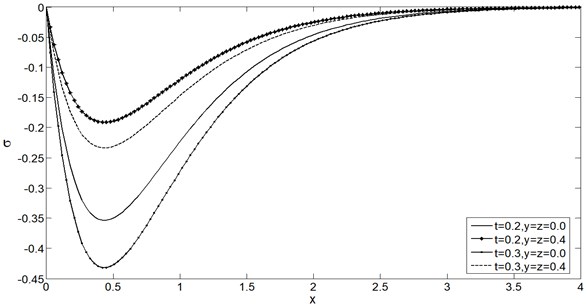
Fig. 7Displacement distribution u vs. x for two time instants

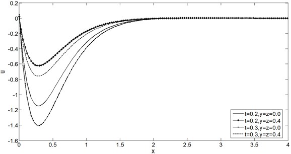
Fig. 8Stress distribution σxx vs. x for two time instants

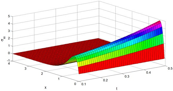
Figs. 9-12 display the temperature $\theta$, the mean stress $\sigma$, the displacement $u$ and the stress ${\sigma }_{xx}$ distributions at $y=z=\mathrm{}$0.4 with wide range of $\text{0}\le x\le \text{0.4}$ and $\text{0.1}\le t\le \text{0.5}$. From these figures it can be noted that the speed of the wave propagation of all the physical quantities are finite and coincide with the physical behaviour of elastic materials. Also we can see from all the figures that the boundary conditions Eqs. (35) and (36) are satisfied.

Fig. 9Temperature distribution θ vs. x and t at y=z= 0.4

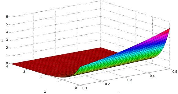
It is clear from Figs. 1-12 that all the distributions considered have a non-zero value only in a bounded region of the space. Outside of this region all the values vanish identically and this means that the region has not felt thermal disturbance yet. Behaviour of all the physical variables at $y=z=\mathrm{}$0.0 and $y=z=\mathrm{}$0.4 are likely to be similar but only differences are lie in the magnitudes.

Fig. 10Mean stress distribution σ vs. x and t at y=z= 0.4

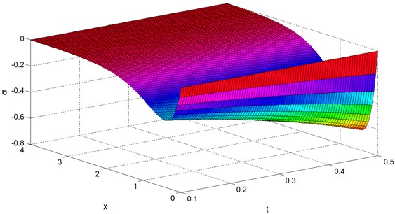
Fig. 11Displacement distribution u vs. x and t at y=z= 0.4

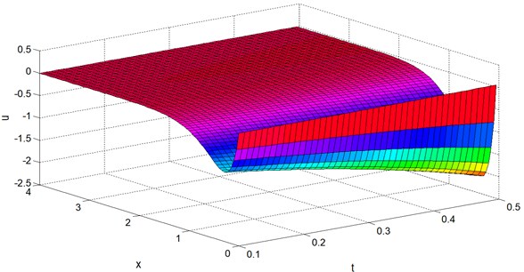
Fig. 12Stress distribution σxx vs. x and t at y=z= 0.4

7. Conclusion

Many researchers in the field of generalized thermoelasticity have applied state-space approach only for one-dimensional thermoelastic problem and very few of them can successfully applied for two-dimensional case. In the present paper, we apply state-space approach for solving a three-dimensional generalized thermoelastic problem for the first time. We tried to implement such a very useful technique which may be applied to solve a three-dimensional generalized thermoviscoelastic problem.