Automation of obtaining initial estimates of reservoir parameters when processing the pressure change curve

1. Introduction

The most useful graph in the analysis of reservoir behavior during well testing is the graph of the derivative of the pressure function. The filtration modes can be determined by studying the shape of the derivative curve in the study of the well by methods of lowering the level and restoring pressure. The formation parameters are calculated on the basis of the pressure data for the corresponding filtration mode. The characteristics of the derivative of the pressure function and the function of the pressure change, manifested over a period of one decade, can be interpreted as one or another flow regime. If the period is shorter than one decade, they most likely represent either noise or a transient process between different filtering modes.

An artificial neural network (NN) can be trained to recognize such distinctive characteristics [5]. In this study, the NN was trained to identify the following 8 patterns: 1) zero slope of the straight line; 2) the unit slope of the straight line; 3) a straight line with a slope; 4) a straight line with a slope; 5) a straight line with a slope; 6) the hump of the curve; 7) dip in the curve; 8) the falling curve.

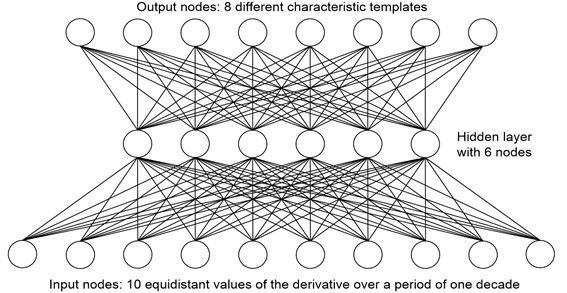
Fig. 1Schematic representation of an artificial NN, used to identify filtration modes

The zero slope pattern of the straight line characterizes the radial flow regimes in an infinite formation and the flow with a single non-conductive discharge. The pattern of a single slope of a straight line at an early and late time after the start of a well test corresponds to flow regimes with the effect of a wellbore and a pseudo-stationary filtration state, respectively. The flow regime in a vertical fracture with finite conductivity is determined by the presence of a straight slope pattern. A direct-slope pattern is used to recognize the flow regime in a vertical fracture with infinite conductivity and/or a linear flow in an elongated formation. Imperfect well (spherical flow) is characterized by a straight sloping pattern. The curve hump pattern is used to identify the transitional period between the borehole effect mode and the radial flow regime in the infinite formation. The filtration in a system with a double porosity corresponds to a pattern of dip in the curve. Finally, the constant pressure regime at the formation boundary can be recognized using a steeply falling curve pattern at the end of the test.

In Fig. 1 is a schematic representation of the artificial NN used [1, 3]. It consists of 10 processing neurons in the input layer, 6 units in the hidden layer and 8 units in the output layer. Each unit in the output layer corresponds to one of the patterns. Since the duration of any template is not less than one decade, the data used for training the National Assembly on the example of all templates was also formed for this period. The decade of training data includes 10 points on the graph of the derivative of the pressure function, evenly distributed in the logarithmic space, because the derivative curve of the pressure function is constructed on a logarithmic scale. The NN is used to test one decade of the well test data at a time. Thus, by moving a “window” with a width of one decade from one point of real data to another, one can identify the template for each of these points.

2. The description of different factors

3. Computational simulations

A flat derivative curve in the flow period in an infinite formation can be recognized by the NN as a zero-slope pattern. The data within the decade that were assigned to the zero-slope pattern was used to plot the graph, where the logarithm of the normal time or Horner time, depending on the type of well test. The straight line was selected by OLS. As already noted, the NN is practically insensitive to noise. Therefore, several graphs were created with different times of beginning and end of the flow in an infinite formation. The starting point was shifted forward in each chart, because The NN sometimes mistakenly adopted the pressure derivative curve as a function of the straight line with zero slope. The end point also shifted in each chart, but already back, because The NN can identify the beginning of a new filtration regime after the flow ends in an infinite reservoir for its continuation. The most probable period of flow in an infinite reservoir was determined by that straight line, which gave the minimum error in the least squares.

Since the trained NN in this study sometimes mistakenly took the peak of the curve hump in a straight line with zero slope, it was necessary to very carefully approach the identification of the present mode of radial flow in an infinite formation. From the practice of interpretation of the well test, it is known that this mode usually manifests itself about a decade and a half after the end of the wellbore effect. Therefore, any flat area that was found before this period was discarded. In some cases, the NN cannot identify any zero-tilt pattern at all. This usually happens if the flat areas were shorter than one decade, or if the data were very noisy. In such cases, it was assumed that the flow period in an infinite formation begins within a decade and a half after the end of the wellbore and lasts for one decade (or less, if the well test has ended earlier). For the selected data, a straight line was selected on a semi-logarithmic scale. Further, several straight lines were aligned on the same scale with different times of the beginning and the end of the flow period in the infinite formation. A straight line with a minimum OLS error was used to calculate permeability and skin factor values.

Since the relationship between the coefficient of elastic capacity of the reservoir $\omega$ and the derivative of the pressure function $t_D{P\text{'}}_D$ is non-linear, the iterative Newton-Raphson procedure was used to calculate the derivative (at the minimum point) for a given value of the derivative $\omega$ [4]. Fig. 2 represents a graph in the logarithmic scale of the elastic capacity coefficient of the reservoir and the derivative of the pressure function, as well as a straight line fitted to this curve. This straight line was used to estimate the initial value of the elastic capacity coefficient of the formation in the Newton-Raphson procedure and is described by the following equation:

Applying the Newton-Raphson procedure, the value $\omega$ can be calculated in this way:

where:

The Newton-Raphson procedure is performed until the absolute difference between ${\omega }_{old}$ and ${\omega }_{new}$ becomes less than some pre-selected deviation. After obtaining the estimate, the estimate can be determined from Eq. (6):

The NN was used to identify the presence of a dip pattern in the curve. The minimum point was determined by comparing the values of the derivative of the pressure function in the vicinity of the dip. If such a template does not exist or was not detected by the NN, then for $\omega$ and $\lambda$ the initial approximation is 0.99.

The experiments were carried out on the collection of real data from the well test in order to assess the effectiveness of the proposed approach.

The well test data used by the pressure reduction method were taken from [6]. In Table 1 shows the values of the parameters of the well and the formation. The well was closed for about 188 hours after more than one year of operation. Since the operating time is long and precisely unknown, the well test was considered as a well test method by lowering the level with a negative flow rate. The derivative of the pressure function and the activation levels for various characteristic patterns are shown in Fig. 3 and 4 respectively.

A single slope pattern (the effect of the wellbore) is present for the first few decades, followed by a hump curve pattern at the same time as the zero slope pattern. The last pattern does not correspond to the true mode of radial flow in an infinite formation, because It is too close to the end of the mode of influence of the wellbore. The current section of the flow in an infinite reservoir is located a decade and a half after the end of the influence mode of the wellbore, but it was not detected by the NN. Nevertheless, one can set this mode using the developed algorithm, which will allow you to calculate the values of permeability and skin factor. After the study of all filtration regimes, initial estimates of formation parameters are determined for the eight reservoir models, the values of which are given in Table 2.

Fig. 2Coefficient of elastic capacity of a layer ω as a function of the pressure derivative tDpD'

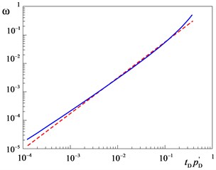
Fig. 3Derived pressure functions at various steps by time in the first study

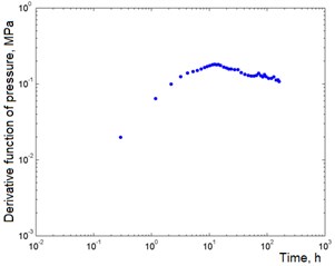
a) Initial time step

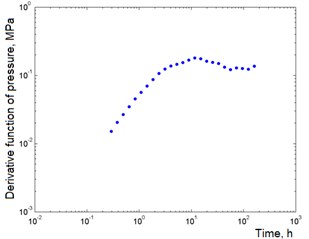
b) Uniform step in line

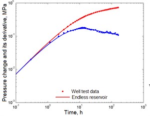
In Fig. 5 is a graph of the derivative of the pressure function with curves matched to the experimental points corresponding to the radial flow model in an infinite formation. The values of the initial and final estimates of the reservoir parameters, as well as the confidence interval values, are summarized in Table 2. It can be seen that these and other estimates are sufficiently close to each other.

Fig. 4Activation levels of different patterns in the first study

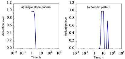
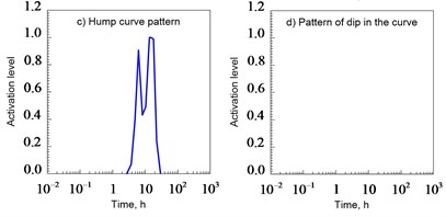
Fig. 5Correspondence of the selected curves to the well test data in the first study

4. Conclusions

1) The NN is not very sensitive to noise in the data. This property is both a virtue and a disadvantage. NN effectively classifies even highly noisy data, without their preliminary smoothing. However, the NN sometimes identified something close, but it was not really a template. Introduction to the algorithm of additional knowledge from the practice of interpretation of well test allowed to minimize false classifications.

2) The NN showed not the best results in recognizing the zero-slope pattern of the straight line. To overcome this problem, it was possible by integrating our knowledge from the field of the well test interpretation and the algorithm for detecting the appropriate filtering mode depending on the output signals of the NN. The use of other NN with their shortcomings may require a change in the procedure for identifying the filtering mode.

3) The proposed approach is aimed at increasing the speed of interpretation of the results of the well test. It is the next step to fully automatic express interpretation of well test based on modern computer facilities. The developed method can also be useful in the framework of automated monitoring of permanent sensors at the bottom of the well.

References

-
Callan Rob Artificial Intelligence. Palgrave, 2003.
Bourdet D. Well Test Analysis: the Use of Advanced Interpretation Models. Elsevier, 2002.
George F. Luger. Artificial Intelligence: Structures and Strategies for Complex Problem Solving, Pearson Education, 2005.
Courant R., Hilbert D. Methods of Mathematical Physics. Interscience Publishers, New York, 1962.
Al-Kaabi A. U., Lee W. J. Using artificial neural nets to identify the well test interpretation model. SPE Formation Evaluation, Vol. 18, Issue 3, 1993, p. 233-240.
Athichanagorn S. Using Artificial Neural Network and Sequential Predictive Probability Method to Mechanize Interpretation of Well Test Data. M.S. Thesis, Stanford University, 1995.
About this article