Abstract
In light of inherent errors associated with the existing methods for predicting lateral spreading of liquefied soil during earthquakes, a novel approach has been proposed. Based on the Newmark sliding block method, a neural network model has been trained to calculate lateral liquefaction displacement, which was achieved by compiling a substantial dataset and establishing a comprehensive seismic motion database. Taking into consideration six input features to train the sensitivity model, based on the sensitivity analysis, a predictive model for liquefaction-induced lateral spreading was developed include three parameters, moment magnitude, peak ground acceleration and yield acceleration. This model was then compared to empirical lateral spreading prediction models. The results demonstrate that this model shows notable concurrence with the existing empirical models. Additionally, using 22 well-documented cases of liquefaction-induced lateral spreading, three high-quality models were employed to predict residual shear strength of the soil. Notably, this novel model surpasses the performance of empirical liquefaction-induced lateral spreading prediction models.
1. Introduction
Liquefaction pertains to the phenomenon in which saturated sandy soil experiences an increase in pore water pressure due to cyclic shearing during an earthquake, subsequently followed by a gradual reduction. The finite deformation of the ground in gentle slope regions is referred to as lateral spreading induced by liquefaction. This lateral spreading can lead to shear failure in pile foundations, resulting in the cracking, stretching, and even collapse of surface structures. The magnitude of lateral spreading influences the seismic design of foundational infrastructure. When lateral spreading is substantial, the impact on engineering facilities becomes notably significant. Hence, the need arises for an accurate predicting method concerning liquefaction-induced lateral spreading.
The Newmark sliding block method, introduced by Newmark in 1965 [1], was initially proposed for computing the permanent displacements of dams subjected to seismic loads. It later found wide application in calculating the permanent displacements of slopes and embankments under earthquake loads. Subsequently, numerous predictive models for lateral spreading based on the Newmark sliding block method have been proposed. For example, Faris et al [2], building upon existing models and utilizing Bayesian regression alongside field and laboratory data, introduced a novel semi-empirical predictive model for liquefaction-induced lateral spreading. Bray and Travasarou [3] based on moment magnitude, yield acceleration, and peak ground acceleration as research parameters. They established a seismic-induced lateral spreading database using 688 seismic records and formulated corresponding displacement prediction models. Jibson [4], through comparative analysis of various parameters including critical acceleration ratio, moment magnitude, Arias intensity, and yield acceleration, employed regression on 2270 seismic records to propose a new displacement prediction model. Rathje and Saygili [5] proposed two displacement prediction models. One relies on a single ground motion parameter (peak ground acceleration), while the other incorporates two ground motion parameters (peak ground acceleration and peak ground velocity), employing a probabilistic approach. Hsieh and Lee [6], relying on plenty of strong earthquake data, introduced a new displacement prediction model through data regression based on Arias intensity and yield acceleration. Ekstrom and Franke [7], incorporating generalized site conditions and lateral spreading reference parameter maps, devised a performance-based probabilistic lateral spreading model for liquefaction induced by earthquakes of recurrence period. Du and Wang [8], employing a probabilistic approach, based one-step lateral spreading prediction model on four seismic parameters, moment magnitude, rupture distance, fault type, and average shear wave velocity of the top 30 meters of soil. Little and Rathje [9], by simulating model geometries numerically, including factors like liquefied soil layer thickness and free surface slope, explored the impact on liquefaction-induced lateral spreading. Consequently, they proposed a bilinear surface model for predicting liquefaction-induced lateral spreading.
In recent years, with the rapid advancement of artificial intelligence and big data technologies, machine learning methods have gained increasing attention and application in the realm of lateral spreading prediction research. Among these methods, algorithms based on machine learning have shown tremendous potential for developing data-driven predictive models [10], [11]. Traditional analytical approaches often require precise function relationships, yet complex seismic phenomena like liquefaction-induced lateral spreading are often challenging to accurately describe using simple mathematical models. Consequently, many researchers have turned to data-driven methods, utilizing machine learning algorithms to uncover patterns and regularities within data and construct corresponding predictive models. For example, Yang et al. [12], utilizing cases of liquefaction-induced lateral spreading, trained an artificial neural network model to predict the residual shear strength ratio of liquefied soil, which is then used for subsequent lateral spreading predictions. Demir and Sahin [13] employed multiple machine learning models including eXtreme Gradient Boosting (XGBoost), Categorical Boosting (CatBoost), and Light Gradient Boosting Machine (LightGBM) to predict liquefaction-induced lateral spreading. They performed comparative analyses using particle swarm optimization and found particle swarm optimization to outperform other models. Gade et al. [14], considering factors such as moment magnitude, seismic source mechanism, and yield acceleration, proposed a new neural network displacement prediction model based on the Newmark sliding block method and a large dataset. This model exhibited good applicability in slope displacement prediction. Kaya et al. [15] compared and analyzed the applicability of multigene genetic programming (MGGP), multilayer perceptron (MLP), and random forest (RF) models in predicting liquefaction-induced lateral spreading. They discovered that the MGGP model provided more accurate predictions for both free-face and gently sloping ground conditions compared to MLP and RF. From the literature, it is evident that machine learning algorithms are capable of swiftly capturing data characteristics and generating predictive values. However, they demand high-quality input data and cannot assess the inherent rationality of the inputs themselves. Therefore, to achieve accurate displacement prediction models, establishing a database with strong and reasonable features for training is of paramount importance.
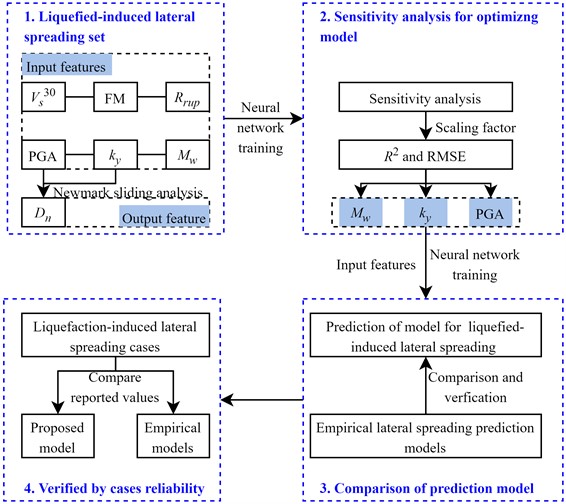
The author has previously evaluated the reliability of applying the Newmark sliding block method to analyze liquefaction-induced lateral spreading [16]. Thus, this paper aims to compute liquefaction-induced lateral spreading values under different yield accelerations based on the Newmark sliding block method. Additionally, based on six input parameters, namely, peak ground acceleration (PGA), yield acceleration (), moment magnitude (), the average shear wave velocity of the top 30 meters of soil (), focal mechanism (FM), and rupture distance (), as well as one output variable, the calculated lateral spreading value, a neural network is employed to train the sensitivity analysis model for lateral spreading parameters. Guided by the outcomes of the sensitivity analysis, three crucial seismic parameters are selected as inputs for training the predictive model of liquefaction-induced lateral spreading. The reliability of this predictive model is evaluated from three different perspectives, i.e., , RMSE, and comparison with empirical prediction models. Furthermore, the applicability of the model is demonstrated through predictions made on well-documented liquefaction-induced lateral spreading cases. The research framework is shown in Fig. 1.
Fig. 1Research framework for prediction of lateral spreading based on Neural network
2. Earthquake motion database and research methods
As previously discussed, machine learning algorithms have the capacity to swiftly capture the features of data and produce predictive outcomes. Nonetheless, these algorithms exhibit a high demand for quality input data and are unable to assess the rationality of the input data. Hence, in this section, an extensive collection of ground seismic records is amassed for the purpose of computing lateral spreading under varying yield accelerations. The calculations are conducted using the Newmark sliding block method.
2.1. Earthquake motion database
A compilation of seismic events has been meticulously collected from various countries, including China, the United States, Canada, Iran, Turkey, and Japan, sourced from the Pacific Earthquake Engineering Research Center [17]. This collection encompasses 27 significant seismic events, among which notable examples are the 1995 Kobe earthquake in Japan, the 1999 Chi-Chi earthquake in Taiwan, and the 1989 Loma Prieta earthquake, amounting to a total of 1960 seismic records. The seismic motion database used for the analysis in this research is detailed in Table 1. Concurrently, corresponding seismic parameters for each event have been systematically gathered and organized. These encompass variables such as PGA, , , FM and .
2.2. Newmark sliding block method
During the soil liquefaction, once liquefaction is triggered and the sliding surface begins to form, the strength of saturated sandy soil rapidly diminishes. As the soil strength continues to decrease, the residual shear strength of the soil remains within the liquefied site. When the shear forces induced by the earthquake, combined with the gravitational forces acting on the soil above the sliding surface, exceed the residual shear strength, the soil above the sliding surface initiates movement. This movement accumulates displacement continuously until the earthquake subsides. The motion pattern of the soil above the sliding surface can be described using the Newmark sliding block method. Specifically, by performing two integrations of the acceleration exceeding the , the resulting displacement under seismic conditions can be determined. The ultimate sliding displacement is the cumulative result of multiple increments of sliding and is illustrated in Fig. 2. This approach has been employed by several scholars to predict lateral spreading induced by liquefaction, including Yang [16], Baziar [18], Taboada [19], Olson, and Johnson [20].
Table 1Ground motion records
No. | Earthquake events | Moment magnitude () | Number of records |
1 | 1940 Imperial Valley, USA | 7 | 2 |
2 | 1952 Kern County, USA | 7.4 | 4 |
3 | 1957 Daly City, USA | 5.3 | 2 |
4 | 1966 Parkfield, USA | 6.2 | 9 |
5 | 1971 San Fernando, USA | 6.6 | 42 |
6 | 1976 Friuli, Italy | 6.5 | 8 |
7 | 1978 Santa Barbara, USA | 5.9 | 4 |
8 | 1978 Tabas, Iran | 7.4 | 8 |
9 | 1979 Coyote Lake, USA | 5.7 | 26 |
10 | 1979 Imperial Valley, USA | 6.5 | 69 |
11 | 1980 Mammoth Lakes, USA | 6.1 | 6 |
12 | 1981 Westmorland, USA | 5.9 | 12 |
13 | 1983 Coalinga, USA | 6.4 | 94 |
14 | 1984 Morgan Hill, USA | 6.2 | 49 |
15 | 1985 Nahanni, Canada | 6.8 | 6 |
16 | 1986 N. Palm Springs, USA | 6.1 | 64 |
17 | 1987 Superstition Hills, USA | 6.5 | 30 |
18 | 1987 Whittier Narrows, USA | 6 | 206 |
19 | 1989 Loma Prieta, USA | 6.9 | 166 |
20 | 1992 Cape Mendocino, USA | 7.1 | 12 |
21 | 1992 Landers, USA | 7.3 | 38 |
22 | 1994 Northridge, USA | 6.7 | 316 |
23 | 1995 Kobe, Japan | 6.9 | 20 |
24 | 1999 Chi-Chi, Taiwan China | 7.6 | 574 |
25 | 1999 Duzce, Turkey | 7.1 | 20 |
26 | 1999 Kocaeli, Turkey | 7.5 | 35 |
27 | 2001 Nisqually, USA | 6.8 | 138 |
Fig. 2Diagram of dynamic permanent displacement calculated by Newmark sliding block method
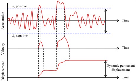
From Fig. 2, it is evident that the is a pivotal parameter in the computation of displacement using the Newmark sliding block method. Therefore, to obtain a substantial dataset of liquefaction-induced lateral spreading calculations suitable for machine learning algorithms, this section assumes various values for the , 0.01 g, 0.03 g, 0.05 g, 0.75 g, 0.1 g, 0.15 g, 0.2 g, 0.25 g, and 0.3 g. The selection range for the is determined based on the analysis of corresponding models using 23 well-documented cases of liquefaction-induced lateral spreading, as compiled by Yang et al. [12]. It is important to note that the computation of necessitates the establishment of a limit equilibrium analysis model based on parameters such as soil distribution, soil strength, soil density, and groundwater levels [16]. Consequently, by employing the , the information encompassing the parameters is inherently considered.
Subsequently, using the collected dataset of 1960 seismic records, lateral spreading under different yield accelerations is computed. Note, before calculating the liquefaction-induced lateral spreading, records with a exceeding the PGA are excluded, as the calculated lateral spreading would be zero. In the end, a total of 8914 valid liquefaction-induced lateral spreading calculations are obtained.
3. Sensitivity analysis model for lateral spreading parameters
By utilizing the Newmark sliding block method for liquefaction-induced lateral spreading calculations, a neural network algorithm is applied to train a sensitivity analysis model for lateral spreading parameters. This involves six seismic parameters, PGA, , , , FM, and , as feature inputs. The () is assigned as the output feature. Subsequently, this neural network model is trained to conduct sensitivity analysis on the factors influencing lateral spreading.
3.1. Parameter selection
Based on the findings from the studies mentioned in references [8] and [14], this research selects six seismic parameters, PGA, , , , FM, and , as input features, with as the output feature. The model used for training the lateral spreading parameter sensitivity analysis is expressed in the following functional form:
where, represents the lateral spreading in mm. PGA stands for peak ground acceleration, measured in units of g, denotes the yield acceleration, also in units of g, signifies the moment magnitude, represents the average shear wave velocity in the top 30 meters of soil, measured in m/s, FM corresponds to the focal mechanism, which includes three forms, i.e., Normal, Reverse, and Strike-Slip faults, and signifies the rupture distance, measured in km.
Table 2The ranges of parameters in the earthquake motion database
Parameter | Range | Unit |
PGA | 0.015-1.779 | g |
0.01-0.30 | g | |
5.3-7.6 | N.A. | |
116-1070 | m/s | |
FM | 1-3 | N.A. |
0.1-100.0 | km |
Within the dataset of 1960 seismic records used in this research, the ranges of the six seismic parameters mentioned above are depicted in Table 2. It is important to note that the is assumed, and in the FM category, 1 corresponds to Normal fault, 2 to Reverse fault, and 3 to Strike-Slip fault. The distribution between PGA and is illustrated in Fig. 3(a), while the distribution among , , and FM is presented in Fig. 3(b).
Fig. 3Distribution of relevant parameters of seismic records [21]
![Distribution of relevant parameters of seismic records [21]](https://static-01.extrica.com/articles/23656/23656-img3.jpg)
a) Distribution of PGA and
![Distribution of relevant parameters of seismic records [21]](https://static-01.extrica.com/articles/23656/23656-img4.jpg)
b) Distribution of , and FM
3.2. Neural network model
A neural network is a type of machine learning algorithm designed to emulate the structure and functionality of the human neural system. It comprises a hierarchical structure of multiple neurons and is utilized for prediction and classification tasks by learning patterns and features from input data. Neural networks optimize model parameters through forward and backward propagation algorithms to minimize prediction errors. A neural network model consists of an input layer, hidden layers, and an output layer. The input layer primarily receives and passes input features to the hidden layers. The hidden layers play a key role in feature extraction and transformation. Finally, the output layer provides the responses of the predictive model.
In this research, there are six input neurons and one output neuron. Additionally, according to the Universal Approximation Theorem, a single hidden layer is sufficient to describe continuous nonlinear functions [14]. Therefore, a single hidden layer is employed. Considering the nonlinear relationship between input and output features, the sigmoid function is chosen as the activation function to produce predicted values that closely approximate input features. The operation stops when the output signal meets the desired criteria; otherwise, error backpropagation is executed. This involves feeding back error values to the hidden layer and continuously adjusting network weights, allowing the hidden layer to gain strong nonlinear mapping capabilities and ultimately produce the desired output. Note, to minimize scale differences between various features and enhance data uniformity, the input features are scaled to a range between -1 and 1 according to Eq. (2):
where, –1 and 1, and and takes the minimum and maximum values of the various features that are mapped.
Based on this framework, 80 % of the data is randomly allocated for training, while the remaining 20 % forms the testing set. Bayesian regularization is employed for training the data. After multiple iterations, the regression achieves the best results with 10 hidden neurons. Thus, the artificial neural network structure employed in this research is depicted in Fig. 4.
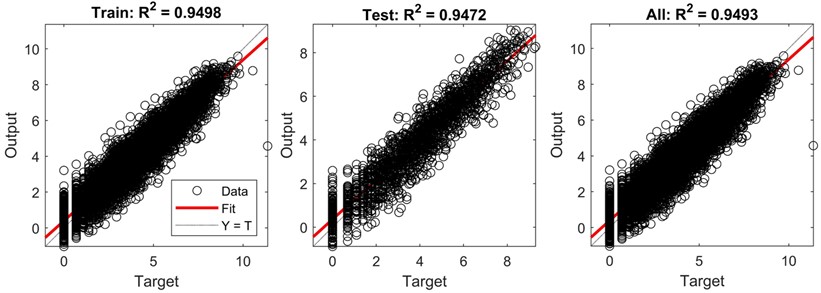
The neural network structure model depicted in Fig. 4 was utilized for training using the dataset from Section 1. Fig. 5 illustrates the performance concerning six parameters related to lateral spreading. Impressively, across the training set, testing set, and the overall assessment, the predicted results consistently exhibit a robust correlation coefficient () of 0.94 or higher. This high and consistent strongly signifies the predictive reliability of the model.
Fig. 4The neural network structure for lateral spreading parameter sensitivity analysis model
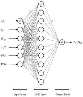
Fig. 5Performance of sensitivity analysis model for liquefaction-induced lateral spreading
3.3. Sensitivity analysis
Considering the challenges in acquiring the six parameters for engineering applications, this study aims to enhance the applicability of the lateral spreading prediction model by conducting a sensitivity analysis. This analysis will compare the influence of the six parameters on the prediction outcomes and identify the three most sensitive parameters to further refine and optimize the model, enhancing its suitability for practical use.
Therefore, all parameters, i.e., PGA, , , , FM, and , were multiplied by scaling factor of 1.2 and 1.5. Using this modified data, a secondary prediction was conducted with the model, and the results were contrasted with the original predictions. Here, taking the PGA as an example is pivotal for illustration. Initially, the PGA undergoes scaling, being amplified by factors of 1.2 and 1.5. Subsequently, leveraging the sensitivity analysis model from Fig. 5, predictions for lateral spreading are made considering the 1.2 and 1.5 scaled PGA while keeping other data constant. Finally, based on the initial lateral spreading predictions, the and RMSE (Root Mean Square Error) are computed separately. This process reveals the and RMSE for each parameter under varying scaling factors. By comparing and RMSE, it becomes possible to assess the sensitivity of the six parameters. This analysis yields the sensitivity of each input feature, as presented in Table 3.
From the variation of and RMSE values in Table 3. It is evident that among the six input parameters, , , and PGA yield the most significant influence on liquefaction-induced lateral spreading. As the energy intensity of an input earthquake is often described by , and PGA, additionally, emerge as a critical factor within the Newmark sliding block frame, representing the input and yield acceleration, respectively. Thus, the three parameters significantly influencing the analysis of lateral spreading [1]:
where, represents the number of observed samples, denotes the th target value, and denotes the th predicted value. RMSE measures the magnitude of deviation between the target values and the predicted values. It reflects the discrepancy between the predicted and actual values.
Table 3Sensitivity analysis of input features [21]
Characteristics | Coefficient of variation | RMSE | |
1.0 | 0.9493 | 0.6962 | |
PGA | 1.2 | 0.9454 | 0.9132 |
1.5 | 0.9304 | 1.3904 | |
1.2 | 0.9455 | 0.9476 | |
1.5 | 0.9248 | 1.8560 | |
1.2 | 0.8613 | 2.0743 | |
1.5 | 0.7256 | 5.7561 | |
1.2 | 0.9469 | 0.7238 | |
1.5 | 0.9347 | 0.8338 | |
FM | 1.2 | 0.9297 | 0.8237 |
1.5 | 0.8821 | 1.0501 | |
1.2 | 0.9468 | 0.7130 | |
1.5 | 0.9380 | 0.7704 |
4. Comparison between the lateral spreading prediction model and the empirical models
In this section, three highly sensitive parameters, identified through sensitivity analysis of liquefaction-induced lateral spreading parameters, are selected as input features to train the lateral spreading prediction model. A subsequent comparison is made with existing empirical models to ascertain the applicability and effectiveness of the model proposed in this research.
4.1. Prediction model of liquefaction-induced lateral spreading
Building upon the original data and the input feature sensitivity analysis results from Table 3, the prediction model is constructed using , , and PGA as input features, with lateral spreading calculated values as the output feature. The functional form of the predictive model is expressed as shown in Eq. (4):
where, it can be observed that this research employs a neural network structure with three input neurons and one output neuron.
Similarly, to account for the nonlinear relationship between seismic parameters and liquefaction-induced lateral spreading, the Sigmoid function is chosen as the activation function for the hidden layer to produce predicted values that approximate the input features. Regarding dataset splitting, the data is randomly divided into an 80 % training set and a 20 % testing set. Bayesian regularization is employed for training the data. After multiple attempts, it was found that the optimal regression performance is achieved with seven hidden neurons.
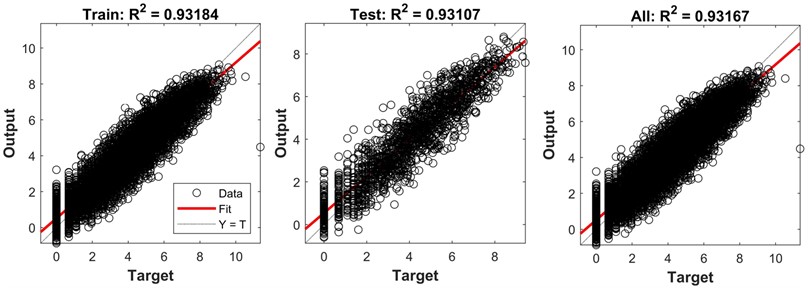
Hence, employing the artificial neural network structure illustrated in Fig. 6, the model was trained to predict lateral spreading. The training results for the lateral spreading prediction model are depicted in Fig. 7. As seen in Fig. 7, whether for the training set, testing set, or overall analysis, the predicted results demonstrate a of 0.93 or higher. This signifies a high level of reliability in the predictive liquefaction-induced lateral spreading of the model.
Fig. 6Neural network structure for liquefaction-induced lateral spreading prediction model
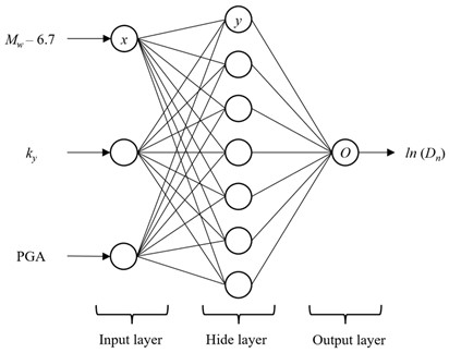
Fig. 7Performance of model for liquefied-induced lateral spreading
4.2. Comparison with empirical lateral spreading prediction models
Upon comparing Fig. 5 and Fig. 7, it becomes evident that the lateral spreading prediction model depicted in Fig. 7 maintains predictive accuracy while halving the number of input parameters, thereby considerably streamlining the model usability. Furthermore, to objectively assess the reliability of the proposed lateral spreading prediction model in this research, a comparative analysis with two established empirical models [4]-[5] that employ identical input variables (, , and PGA) was conducted. This comparative analysis serves to offer additional insights into the model proposed in this research.
It is worth noting that the Jibson 2007 model [4] is applicable for 5.3 ≤ ≤ 7.6. Therefore, to align with the constraints outlined in references [4]-[5] and the proposed model in this research, the specified ranges for , , and PGA are as follows, 5.3 ≤ ≤ 7.6, 0.01 ≤ ≤ 0.30 g, 0.015 ≤ PGA ≤ 1.779 g, as depicted in Fig. 8.
1. Jibson 2007 model [4], referred to as J07:
2. Rathje and Saygili 2009 model [5], abbreviated as RS09:
In Eqs. (5-6), represents the lateral spreading in cm.
Fig. 8Comparison of the lateral spreading predictions model with the existing empirical prediction models [21]
![Comparison of the lateral spreading predictions model with the existing empirical prediction models [21]](https://static-01.extrica.com/articles/23656/23656-img9.jpg)
a) Variation with respect to with 0.15g, PGA = 0.3 g
![Comparison of the lateral spreading predictions model with the existing empirical prediction models [21]](https://static-01.extrica.com/articles/23656/23656-img10.jpg)
b) Variation with respect to with 7.0, PGA = 0.3 g
![Comparison of the lateral spreading predictions model with the existing empirical prediction models [21]](https://static-01.extrica.com/articles/23656/23656-img11.jpg)
c) Variation with respect to PGA with 7.0, 0.15 g
From Fig. 8(a), it can be observed that for constant values of other seismic parameters, as the increases, the lateral spreading also increases. This is because a larger implies higher energy carried by seismic waves during the corresponding seismic event, making liquefaction-prone areas more susceptible to liquefaction, resulting in larger lateral spreading.
In Fig. 8(b), it is evident that with constant values for other seismic parameters, an increase in the results in a decrease in the lateral spreading. This observation aligns with the displacement calculation theory of Newmark [1], where, under unchanged conditions, a higher leads to a smaller Newmark-calculated displacement. Moreover, a higher signifies a greater residual shear strength of liquefied soil. Soil displacement begins only when the combined shear forces resulting from seismic and gravitational effects surpass the residual shear strength. As a result, the lateral spreading decreases.
Fig. 8(c) illustrates that different PGA have varying effects on liquefaction-induced lateral spreading. However, there is an overall trend of increasing lateral spreading with higher PGA, like the pattern observed for moment magnitude. This alignment with theoretical expectations and the calculation principles of Newmark [1] reinforces the consistency of the model.
The alignment of the proposed predictive model with theoretical analysis and its good agreement with existing empirical models highlight its reliability. This suggests that the proposed liquefaction-induced lateral spreading prediction model can effectively capture the intricate nonlinear relationship between input parameters and the output parameter, making it a dependable prediction tool.
5. Example application of liquefaction-induced lateral spreading
To further validate the reliability of the proposed model for lateral spreading prediction, this section gathers and organizes a dataset of 22 well-cases of lateral spreading. This dataset will be utilized for validation analysis. The observed data of lateral spreading serve as the benchmark to evaluate the effectiveness of the methodology presented in this research. Additionally, a comparative analysis will be conducted by comparing the predictions of the proposed model with those of existing empirical models.
5.1. Example of lateral spreading of liquefaction
A comprehensive dataset of liquefaction-induced lateral spreading well-cases has been meticulously gathered and organized for validation based on published literature. This dataset encompasses detailed information about soil profiles, soil properties, and Standard Penetration Test (SPT) values of potentially liquefiable soils. The collected data has been compiled into an extensive lateral spreading database, as presented in Table 4. This table incorporates various parameters, including (N1)60, which signifies the normalized and standardized SPT blow count under standard atmospheric pressure, and (N1)60-cs, representing the equivalent clean-sand normalized SPT blow count, accounting for the purity of the sand. Additionally, denotes the natural logarithm of the observed lateral spreading in the field, measured in millimeters (mm).
Table 4Basic information of lateral spreading example [16]
No. | Earthquake event | Site | PGA | (N1)60 | (N1)60-cs | Ref. | |
1 | 6.6, San Fernando, US, 1971 | Juvenile hall | 0.7 | 6.9 | 9.7 | 7.313 | [22] |
2 | 6.5, Imperial Valley, US, 1979 | Heber Road | 0.8 | 1 | 2.7 | 7.650 | [23], [24] |
3 | 6.9, Borah Peaks, US, 1983 | Whiskey Springs fan | 0.6 | 13 | 14.8 | 6.620 | [25] |
4 | 6.6, Superstition Hills, US, 1987 | Wildlife Site | 0.21 | 10.3 | 12.7 | 5.193 | [26], [27] |
5 | 7.0, Loma Prieta, US, 1989 | Moss Landing Bldg4 | 0.25 | 10 | 10.5 | 5.635 | [28] |
6 | Moss Landing Bldg3 | 0.25 | 10 | 10.1 | 5.521 | [28] | |
7 | MLML eastward (A-A) | 0.25 | 14.6 | 15 | 6.109 | [29] | |
8 | MLML eastward (B-B) | 0.25 | 14.6 | 15 | 6.109 | [29] | |
9 | Leonardini Farm | 0.16 | 4.3 | 5.1 | 5.521 | [30] | |
10 | Treasure island | 0.16 | 10 | 11 | 5.521 | [31] | |
11 | 7.4, Manjil, Iran, 1990 | Rudbanch town canal | 0.15 | 8.63 | 9.1 | 6.908 | [32] |
12 | 6.7, Northridge, US, 1994 | Wynne Ave | 0.51 | 11.6 | 14.2 | 5.011 | [19], [33] |
13 | 7.6, Chi-Chi, Taiwan (China), 1999 | Wufeng Site C (A-A) | 0.81 | 3.5 | 6.5 | 7.626 | [34] |
14 | Wufeng Site C (B-B) | 0.81 | 3.5 | 5.3 | 6.194 | [34] | |
15 | Wufeng Site C1 | 0.81 | 14.5 | 16.3 | 7.123 | [34] | |
16 | Wufeng Site B | 0.81 | 10 | 11.8 | 7.993 | [34] | |
17 | Wufeng Site M | 0.81 | 11.5 | 12.6 | 7.390 | [34] | |
18 | Nantou Site N | 0.42 | 9 | 10.4 | 5.521 | [34] | |
19 | 7.4, Kocaeli, Turkey, 1999 | Hotel Sapanca | 0.4 | 13.4 | 14.1 | 7.601 | [35] |
20 | Police Station | 0.4 | 5 | 7 | 7.783 | [36] | |
21 | Soccer Field | 0.4 | 7 | 9.7 | 7.090 | [36] | |
22 | Yalova Harbor | 0.3 | 14.53 | 16.3 | 5.704 | [36] |
5.2. Application of lateral spreading prediction model
The determination of the yield acceleration for lateral spreading involves various factors, including soil layer distribution, soil strength, soil unit weight, and groundwater level. To achieve this, a limit equilibrium analysis model is set up using Slide software, utilizing the Morgenstern-Price method for limit equilibrium analysis. A critical step in this process is establishing the residual shear strength of the liquefiable soil, as emphasized by previous research [16].
To calculate the residual shear strength of the liquefiable soil, three different formulas are utilized, i.e., Olson and Johnson [20], Idriss and Boulanger [37], and Kramer and Wang [38]. These formulas are applied based on the standard penetration test (SPT) values of the liquefiable soil. By adjusting the dynamic load factor to achieve a safety factor of exactly 1.0, corresponding to the horizontal seismic coefficient, the yield acceleration of the site is obtained. The yield accelerations determined using different residual shear strength prediction models are summarized in Table 5. This process ensures that the analysis captures the specific characteristics of the liquefaction potential of the soil in question.
Table 5Residual shear strength and yield acceleration of liquefied soil in different models
No. | Site | Residual shear strength (kPa) | Yield acceleration (g) | ||||
Ref. [20] | Ref. [37] | Ref. [38] | Ref. [20] | Ref. [37] | Ref. [38] | ||
1 | Juvenile hall | 7.04 | 8.25 | 8.02 | 0.072 | 0.08 | 0.076 |
2 | Heber Road | 2.32 | 2.85 | 3.69 | 0.004 | 0.006 | 0.021 |
3 | Whiskey Springs fan | 13.69 | 22.22 | 16.78 | 0.07 | 0.16 | 0.095 |
4 | Wildlife Site | 6.61 | 6.76 | 9.52 | 0.028 | 0.03 | 0.07 |
5 | Moss Landing Bldg4 | 6.69 | 6.66 | 9.39 | 0.007 | 0.007 | 0.08 |
6 | Moss Landing Bldg3 | 8.82 | 8.4 | 10.84 | 0.017 | 0.013 | 0.056 |
7 | MLML eastward (A-A) | 10.03 | 15.58 | 15.97 | 0.095 | 0.159 | 0.175 |
8 | MLML eastward (B-B) | 19.51 | 30.13 | 22.81 | 0.165 | 0.24 | 0.19 |
9 | Leonardini Farm | 1.87 | 1.8 | 3.6 | 0.15 | 0.15 | 0.2 |
10 | Treasure Island | 4.62 | 4.87 | 7.79 | 0.05 | 0.055 | 0.095 |
11 | Rudbanch town canal | 22.03 | 20.92 | 16.3 | 0.036 | 0.036 | 0.02 |
12 | Wynne Ave | 14.54 | 22.79 | 15.74 | 0.1 | 0.152 | 0.11 |
13 | Wufeng Site C (A-A) | 4.51 | 5.55 | 5.45 | 0.08 | 0.09 | 0.09 |
14 | Wufeng Site C (B-B) | 4.55 | 4.96 | 5.47 | 0.12 | 0.13 | 0.14 |
15 | Wufeng Site C1 | 10.65 | 10.59 | 16.36 | 0.105 | 0.105 | 0.17 |
16 | Wufeng Site B | 7.1 | 6.99 | 9.68 | 0.05 | 0.05 | 0.1 |
17 | Wufeng Site M | 6.96 | 8.21 | 10.59 | 0.05 | 0.075 | 0.09 |
18 | Nantou Site N | 2.98 | 2.87 | 5.89 | 0.06 | 0.057 | 0.12 |
19 | Hotel Sapanca | 4.68 | 5.31 | 4.74 | 0.04 | 0.06 | 0.045 |
20 | Police Station | 2.5 | 2.15 | 3.86 | 0.02 | 0.006 | 0.08 |
21 | Soccer Field | 3.59 | 3.04 | 5.06 | 0.135 | 0.126 | 0.17 |
22 | Yalova Harbor | 11.4 | 11.28 | 16.99 | 0.083 | 0.08 | 0.16 |
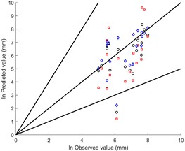
The application of the model proposed in this research is compared with the Jibson 2007 model [4] and the Rathje and Saygili 2009 model [5]. Using the residual shear strength predictions from the Olson and Johnson [20], Idriss and Boulanger [37], and Kramer and Wang [38] models, the lateral spreading for the 22 liquefaction cases described in Table 5 are predicted. These predictions are compared with observed lateral spreading data to assess the effectiveness of the proposed method. The predictive results are illustrated in Fig. 9.
To provide an objective assessment of the accuracy of the lateral spreading prediction method presented in this research, the evaluation is conducted using and RMSE. The results are detailed in Table 6. This comprehensive analysis aims to validate the reliability and accuracy of the approach outlined in this research when compared to established models and actual observations.
Upon examining the evaluation metrics presented in Table 6, it is evident that the proposed method in this research consistently outperforms the Jibson 2007 model and the Rathje and Saygili 2009 model across most cases. Notably, when utilizing the residual shear strength predictions by Kramer and Wang [38], the performance of the proposed method is marginally lower than that of the Jibson 2007 model. However, in the remaining scenarios, the proposed method surpasses both the Jibson 2007 model and the Rathje and Saygili 2009 model. This comparative analysis underscores the effectiveness and accuracy of the approach developed in this research for predicting lateral spreading.
Fig. 9Prediction of liquefaction-induced lateral spreading based on different residual shear strength models of liquefied soil
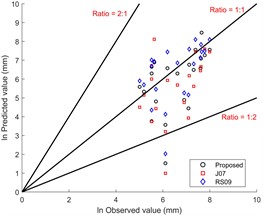
a) Olson and Johnson model [20]
b) Idriss and Boulanger model [37]
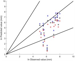
c) Kramer and Wang model [38]
Table 6Application of prediction model for lateral spreading
Model of residual shear strength | Prediction method | Evaluation index | |
RMSE | |||
Olson and Johnson [20] | Proposed | 0.500 | 2.020 |
J07 [4] | 0.471 | 2.672 | |
RS09 [5] | 0.474 | 2.150 | |
Idriss and Boulanger [37] | Proposed | 0.477 | 2.455 |
J07 [4] | 0.431 | 3.521 | |
RS09 [5] | 0.439 | 2.824 | |
Kramer and Wang [38] | Proposed | 0.582 | 2.900 |
J07 [4] | 0.639 | 2.867 | |
RS09 [5] | 0.431 | 5.337 | |
6. Conclusions
This research developed a predictive model for lateral spreading induced by liquefaction using a data-driven approach. The model is built on artificial neural networks and machine learning techniques, enabling accurate predictions of lateral spreading given specific seismic parameters. Through a sensitivity analysis, it was identified that the most influential seismic parameters, and they were incorporated into the model construction, leading to further enhancement of prediction applicability. Compared to existing empirical models, the proposed model demonstrates great performance in predicting liquefaction-induced lateral spreading. The following conclusions and suggestions have been drawn.
1) Neural networks were able to capture the nonlinear relationships between input and output features, which was proved in predicting liquefaction-induced lateral spreading. Based on sensitivity analysis, moment magnitude, yield acceleration, and peak ground acceleration are critical factors for an accurate lateral spreading prediction. The liquefaction-induced lateral spreading prediction model trained in this research demonstrates great performance compared to empirical models across 22 well-documented cases of liquefaction-induced lateral spreading.
2) It should be emphasized that exploring alternative neural network structures or basis functions may potentially yield even greater improvements in accurately predicting liquefaction-induced lateral spreading.
References
-
N. M. Newmark, “Effects of earthquakes on dams and embankments,” Géotechnique, Vol. 15, No. 2, pp. 139–160, Jun. 1965, https://doi.org/10.1680/geot.1965.15.2.139
-
Allison T. Faris, Raymond B. Seed, Robert E. Kayen, and Jiaer Wu, “A semi-empirical model for the estimation of maximum horizontal displacement due to liquefaction-induced lateral spreading,” in 8th U.S. National Conference of Earthquake Engineering, pp. 1584–1593, Jan. 2006.
-
J. D. Bray and T. Travasarou, “Simplified procedure for estimating earthquake-induced deviatoric slope displacements,” Journal of Geotechnical and Geoenvironmental Engineering, Vol. 133, No. 4, pp. 381–392, Apr. 2007, https://doi.org/10.1061/(asce)1090-0241(2007)133:4(381)
-
R. W. Jibson, “Regression models for estimating coseismic landslide displacement,” Engineering Geology, Vol. 91, No. 2-4, pp. 209–218, May 2007, https://doi.org/10.1016/j.enggeo.2007.01.013
-
E. M. Rathje and G. Saygili, “Probabilistic assessment of earthquake-induced sliding displacements of natural slopes,” Bulletin of the New Zealand Society for Earthquake Engineering, Vol. 42, No. 1, pp. 18–27, Mar. 2009, https://doi.org/10.5459/bnzsee.42.1.18-27
-
S.-Y. Hsieh and C.-T. Lee, “Empirical estimation of the Newmark displacement from the Arias intensity and critical acceleration,” Engineering Geology, Vol. 122, No. 1-2, pp. 34–42, Sep. 2011, https://doi.org/10.1016/j.enggeo.2010.12.006
-
L. T. Ekstrom and K. W. Franke, “Simplified procedure for the performance-based prediction of lateral spread displacements,” Journal of Geotechnical and Geoenvironmental Engineering, Vol. 142, No. 7, p. 04016, Jul. 2016, https://doi.org/10.1061/(asce)gt.1943-5606.0001440
-
W. Du and G. Wang, “A one-step Newmark displacement model for probabilistic seismic slope displacement hazard analysis,” Engineering Geology, Vol. 205, pp. 12–23, Apr. 2016, https://doi.org/10.1016/j.enggeo.2016.02.011
-
M. Little and E. Rathje, “Key trends regarding the effects of site geometry on lateral spreading displacements,” Journal of Geotechnical and Geoenvironmental Engineering, Vol. 147, No. 12, p. 04021, Dec. 2021, https://doi.org/10.1061/(asce)gt.1943-5606.0002690
-
W. Zhang, X. Gu, L. Tang, Y. Yin, D. Liu, and Y. Zhang, “Application of machine learning, deep learning and optimization algorithms in geoengineering and geoscience: Comprehensive review and future challenge,” Gondwana Research, Vol. 109, pp. 1–17, Sep. 2022, https://doi.org/10.1016/j.gr.2022.03.015
-
C. Qin, W. Zhao, K. Zhong, and W. Chen, “Prediction of longwall mining‐induced stress in roof rock using LSTM neural network and transfer learning method,” Energy Science and Engineering, Vol. 10, No. 2, pp. 458–471, Dec. 2021, https://doi.org/10.1002/ese3.1037
-
Y. Yang, B. Yang, C. Su, and J. Ma, “Application of residual shear strength predicted by artificial neural network model for evaluating liquefaction-induced lateral spreading,” Advances in Civil Engineering, Vol. 2020, pp. 1–15, Aug. 2020, https://doi.org/10.1155/2020/8886781
-
S. Demir and E. K. Sahin, “Predicting occurrence of liquefaction-induced lateral spreading using gradient boosting algorithms integrated with particle swarm optimization: PSO-XGBoost, PSO-LightGBM, and PSO-CatBoost,” Acta Geotechnica, Vol. 18, No. 6, pp. 3403–3419, Jan. 2023, https://doi.org/10.1007/s11440-022-01777-1
-
M. Gade, P. S. Nayek, and J. Dhanya, “A new neural network-based prediction model for Newmark’s sliding displacements,” Bulletin of Engineering Geology and the Environment, Vol. 80, No. 1, pp. 385–397, Aug. 2020, https://doi.org/10.1007/s10064-020-01923-7
-
Z. Kaya, L. Latifoglu, E. Uncuoglu, A. Erol, and M. S. Keskin, “Predicting liquefaction-induced lateral spreading by using the multigene genetic programming (MGGP), multilayer perceptron (MLP), and random forest (RF) techniques,” Bulletin of Engineering Geology and the Environment, Vol. 82, No. 3, pp. 1–18, Feb. 2023, https://doi.org/10.1007/s10064-023-03103-9
-
Y. Yang and E. Kavazanjian, “Newmark analysis of lateral spreading induced by liquefaction,” Journal of Earthquake Engineering, Vol. 26, No. 6, pp. 3034–3053, Apr. 2022, https://doi.org/10.1080/13632469.2020.1784316
-
T. D. Ancheta et al., “NGA-West2 database,” Earthquake Spectra, Vol. 30, No. 3, pp. 989–1005, Aug. 2014, https://doi.org/10.1193/070913eqs197m
-
M. H. Baziar, R. Dobry, and A.-W. M. Elgamal, “Engineering evaluation of permanent ground deformations due to seismically induced liquefaction,” 1992.
-
V. M. Taboada-Urtuzuástegui, F. J. Villegas-Rodríguez, and F. Hernández-Martinez, “Prediction of lateral displacements induced by liquefaction in the Port of Manzanillo, Mexico during the earthquake of October 9, 1995,” in International Conferences on Recent Advances in Geotechnical Earthquake Engineering and Soil Dynamics, 2001.
-
S. M. Olson and C. I. Johnson, “Analyzing liquefaction-induced lateral spreads using strength ratios,” Journal of Geotechnical and Geoenvironmental Engineering, Vol. 134, No. 8, pp. 1035–1049, Aug. 2008, https://doi.org/10.1061/(asce)1090-0241(2008)134:8(1035)
-
Y. Yang, Z. Lin, H. Lu, and X. Zhan, “Prediction model of lateral spreading of liquefied soil during earthquakes based on neural network,” Vibroengineering Procedia, Vol. 51, pp. 42–48, Oct. 2023, https://doi.org/10.21595/vp.2023.23541
-
M. Hudson, I. Idriss, and M. Beikae, “QUAD4M – a computer program to evaluate the seismic response of soil structures using finite element procedures incorporating a compliant base,” University of California, 1994.
-
G. Castro, “Empirical methods in liquefaction evaluation,” in 1st Annual Leonardo Zeevaert International Conference, 1995.
-
T. L. Youd and M. J. Bennett, “Liquefaction sites, Imperial Valley, California,” Journal of Geotechnical Engineering, Vol. 109, No. 3, pp. 440–457, Mar. 1983, https://doi.org/10.1061/(asce)0733-9410(1983)109:3(440)
-
R. D. Andrus and T. L. Youd, “Subsurface investigation of a liquefaction-induced lateral spread, Thousand Springs Valley, Idaho,” Geotechnical Laboratory, 1987.
-
T. L. Holzer, T. C. Hanks, and T. L. Youd, “Dynamics of Liquefaction during the 1987 Superstition Hills, California, Earthquake,” Science, Vol. 244, No. 4900, pp. 56–59, Apr. 1989, https://doi.org/10.1126/science.244.4900.56
-
R. W. Boulanger, D. W. Wilson, and I. M. Idriss, “Examination and reevalaution of SPT-based liquefaction triggering case histories,” Journal of Geotechnical and Geoenvironmental Engineering, Vol. 138, No. 8, pp. 898–909, Aug. 2012, https://doi.org/10.1061/(asce)gt.1943-5606.0000668
-
R. W. Boulanger, L. H. Mejia, and I. M. Idriss, “Liquefaction at moss landing during Loma Prieta earthquake,” Journal of Geotechnical and Geoenvironmental Engineering, Vol. 123, No. 5, pp. 453–467, May 1997, https://doi.org/10.1061/(asce)1090-0241(1997)123:5(453)
-
L. H. Mejia, “Liquefaction at Moss Landing,” Washington, U.S. Geological Survey, 1998.
-
C. W. A. Charlie et al., “Direct measurement of liquefaction potential in soils of Monterey County, California,” Colorado, U.S. Geological Survey, 1998.
-
H. Lu, Z. Lin, X. Zhan, Y. Yang, and D. Wu, “Numerical simulation of seismic liquefaction for treasure island site,” Lecture Notes in Civil Engineering, pp. 407–415, May 2023, https://doi.org/10.1007/978-981-99-1748-8_36
-
M. K. Yegian, V. G. Ghahraman, M. A. A. Nogole-Sadat, and H. Daraie, “Liquefaction during the 1990 Manjil, Iran, earthquake, II: Case history analyses,” Bulletin of the Seismological Society of America, Vol. 85, No. 1, pp. 83–92, Feb. 1995, https://doi.org/10.1785/bssa0850010083
-
T. L. Holzer, “Liquefaction and soil failure during 1994 Northridge earthquake,” Journal of Geotechnical and Geoenvironmental Engineering, Vol. 125, No. 6, pp. 438–452, Jan. 1999.
-
D. B. Chu, J. P. Stewart, T. L. Youd, and B. L. Chu, “Liquefaction-induced lateral spreading in near-fault regions during the 1999 Chi-Chi, Taiwan earthquake,” Journal of Geotechnical and Geoenvironmental Engineering, Vol. 132, No. 12, pp. 1549–1565, Dec. 2006, https://doi.org/10.1061/(asce)1090-0241(2006)132:12(1549)
-
K. O. Cetin et al., “Liquefaction-induced ground deformations at Hotel Sapanca during Kocaeli (Izmit), Turkey earthquake,” Soil Dynamics and Earthquake Engineering, Vol. 22, No. 9-12, pp. 1083–1092, Oct. 2002, https://doi.org/10.1016/s0267-7261(02)00134-3
-
K. O. Cetin et al., “Liquefaction-induced lateral spreading at Izmit Bay During the Kocaeli (Izmit)-Turkey earthquake,” Journal of Geotechnical and Geoenvironmental Engineering, Vol. 130, No. 12, pp. 1300–1313, Dec. 2004, https://doi.org/10.1061/(asce)1090-0241(2004)130:12(1300)
-
I. M. Idriss and R. W. Boulanger, “SPT – and CPT-based relationships for the residual shear strength of liquefied soils,” in Geotechnical, Geological and Earthquake Engineering, pp. 1–22, Sep. 2023, https://doi.org/10.1007/978-1-4020-5893-6_1
-
S. L. Kramer and C.-H. Wang, “Empirical model for estimation of the residual strength of liquefied soil,” Journal of Geotechnical and Geoenvironmental Engineering, Vol. 141, No. 9, p. 04015, Sep. 2015, https://doi.org/10.1061/(asce)gt.1943-5606.0001317
About this article

This research was supported by Innovation Project of Guangxi Graduate Education (No. YCSW2023297).
The datasets generated during and/or analyzed during the current study are available from the corresponding author on reasonable request.
Yanxin Yang conceived the research study and provided input for revisions. Ziyun Lin designed the algorithms and drafted the initial manuscript. Hua Lu, Xudong Zhan and Shihui Ma collected and organized information.
The authors declare that they have no conflict of interest.
