Abstract
In response to the complex issue of predicting lateral spreading of liquefied soil during earthquakes, this study establishes a comprehensive seismic database. The Newmark sliding block method is utilized to calculate lateral displacements, and a sensitivity analysis model for liquefaction-induced lateral spreading is developed by considering multiple parameters. Based on the three most influential parameters identified through sensitivity analysis, a novel liquefaction-induced lateral spreading prediction model is proposed. The reliability of this new model is then demonstrated by comparing it with existing classical prediction models, as well as by analyzing correlation coefficients and root mean square errors.
Highlights
- A neural network-based prediction model that effectively captures complex relationships between input parameters and liquefaction-induced lateral spreading.
- Moment magnitude, yield acceleration, and peak ground acceleration are identified as the most influential factors in predicting lateral spreading.
- The newly proposed prediction model demonstrates reliability by aligning well with existing classical models and exhibiting strong correlation coefficients.
1. Introduction
Liquefaction refers to the phenomenon where saturated sandy soil experiences an increase in pore water pressure due to cyclic shear during an earthquake, leading to continuous reduction in strength. The lateral spreading of the ground caused by liquefaction is a typical form of damage in seismic areas. This lateral spreading can result in shear failure of pile foundations and cause cracking, stretching, and even collapse of ground structures. The magnitude of lateral spreading can significantly impact the seismic design of infrastructure. When lateral spreading displacement is significant, it can cause considerable damage to engineering facilities. Therefore, it is essential to propose an accurate prediction method for liquefaction-induced lateral spreading.
In recent years, with the rapid development of artificial intelligence and big data technology, machine learning methods in lateral spreading prediction research have gained increasing attention and application. Among them, algorithms based on machine learning have shown great potential in developing data-driven predictive models [1]. Traditional analytical methods often require precise functional relationships, however, complex seismic problems like lateral spreading are difficult to accurately describe using simple mathematical models. Therefore, many researchers have turned to data-driven approaches, utilizing machine learning algorithms to discover patterns and regularities in data and build corresponding predictive models. For instance, Yang et al. [2] trained an artificial neural network model based on lateral spreading examples to predict the residual shear strength ratio of liquefied soil, which is used for subsequent lateral spreading prediction. Demir and Sahin [3] utilized multiple machine learning models, such as eXtreme Gradient Boosting, Categorical Boosting, and Light Gradient Boosting Machine, to predict lateral spreading values and compared them using the particle swarm optimization algorithm, finding that the particle swarm optimization algorithm outperformed other models. Gade et al. [4] considered factors like moment magnitude, focal mechanism, and yield acceleration, and proposed a new neural network displacement prediction model based on the Newmark sliding block method using a large amount of data, demonstrating its good applicability in slope displacement prediction. Kaya et al. [5] compared the applicability of multigene genetic programming, multilayer perceptron, and random forest models in lateral spreading prediction, and found that the MGGP model was more accurate in predicting lateral spreading values for free-face and gently sloping ground compared to MLP and RF. From the aforementioned literature, it can be observed that machine learning algorithms can quickly grasp the characteristics of data and output predictions. However, they require high-quality input data and cannot judge the reasonableness of the input data itself. Therefore, in order to obtain accurate displacement prediction models, it is crucial to establish a strong and reasonable database for training.
The Newmark sliding block method was first proposed by Newmark [6] in 1965 for calculating the permanent displacement of dams under seismic loads. It has since been widely used to compute the permanent displacement of slopes and embankments under earthquake loads. The author has already evaluated the reliability of the Newmark sliding block method for analyzing lateral spreading [7]. Therefore, the purpose of this study is to use the Newmark sliding block method to calculate the lateral spreading values under different yield accelerations. Additionally, based on 6 input parameters, namely, peak ground acceleration (PGA), yield acceleration (), moment magnitude (), the average shear wave velocity of the top 30 meters of soil (), focal mechanism (FM), and rupture distance (), as well as 1 output variable, the calculated lateral spreading value, a neural network is employed to train the sensitivity analysis model for lateral spreading parameters, facilitating the sensitivity analysis of each parameter. Utilizing the results of the sensitivity analysis, 3 critical seismic parameters are selected as inputs to train the lateral spreading prediction model. The reliability of this model is assessed from three different perspectives, , RMSE, and classical prediction models.
2. Earthquake motion database and research methods
In this study, a seismic motion database consisting of 1960 records from 27 earthquake events was collected and compiled from various countries such as China, the United States, Canada, Iran, Turkey, and Japan. Some of the notable earthquakes included the 1995 Kobe earthquake in Japan, the 1999 Chi-Chi earthquake in Taiwan (China), and the 1989 Loma Prieta earthquake, among others. The seismic motion database was obtained from the PEER-NGA-West2 database [8]. Additionally, relevant seismic parameters were gathered for each earthquake event, including peak ground acceleration, moment magnitude, and rupture distance. It is important to note that the selected seismic records are all from surface horizontal ground motion, encompassing both EW (East-West) and NS (North-South) directions, and both directions are considered as independent seismic records for analysis.
As previously mentioned, machine learning algorithms can quickly learn the features of data and generate predictive results. However, these algorithms have higher demands for input data and cannot assess the reasonableness of the input data. Therefore, in this section, to obtain a large number of liquefaction-induced lateral displacement values suitable for machine learning algorithms, we assume different yield accelerations, specifically 0.01 g, 0.03 g, 0.05 g, 0.75 g, 0.1 g, 0.15 g, 0.2 g, 0.25 g, and 0.3 g. It is important to note that the selection of the range of yield accelerations is based on the analysis of corresponding models as determined by Yang et al. [2] in their compilation of 23 verified liquefaction-induced lateral displacement instances. Moreover, the calculation of yield acceleration requires the establishment of a limit equilibrium analysis model based on parameters such as soil distribution, soil strength, soil density, and groundwater level [7]. Therefore, by considering yield acceleration, we implicitly account for the information from the aforementioned parameters.
Based on this, using the collected 1960 seismic records, liquefaction-induced lateral displacement values are calculated for different yield accelerations. It is important to note that before calculating the lateral displacement values, records with yield accelerations greater than the peak ground acceleration are excluded. This is because if this condition is not met, the calculated lateral displacement value would be zero. As a result, 8914 valid liquefaction-induced lateral displacement values are obtained after applying this condition.
3. Sensitivity analysis model for liquefaction lateral movement parameters
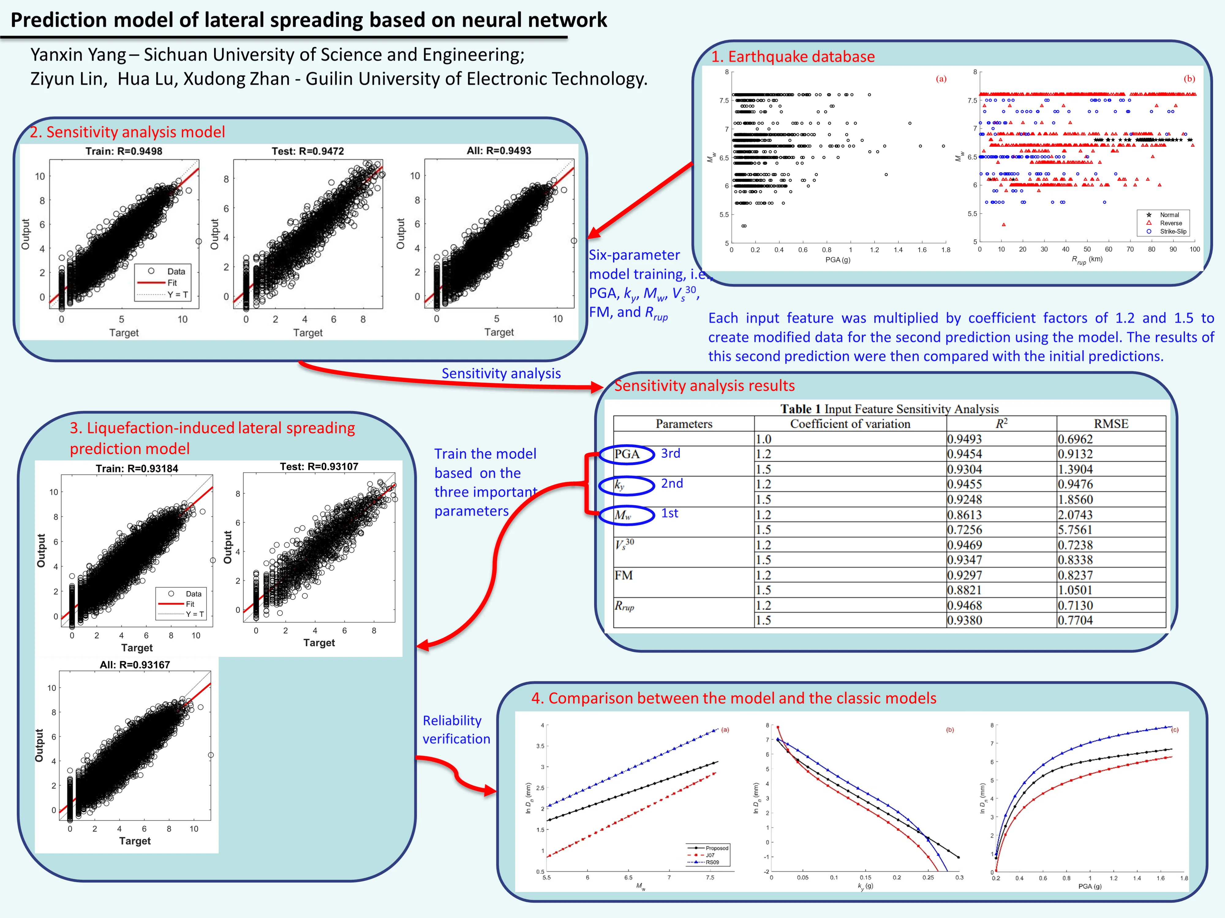
Based on the research findings from references [4], [9], this study selects six seismic parameters, namely PGA, , , , FM, and , as feature inputs. The ln () is used as the output parameter for training the lateral displacement parameter analysis model. The distribution of PGA and is shown in Fig. 1(a), while the distribution of , and FM is depicted in Fig. 1(b). From Fig. 1, it is evident that the seismic parameter ranges are 0.015 ≤ PGA ≤ 1.779 g, 0.01 ≤ ≤ 0.30g, 5.3 ≤ ≤ 7.6, 116 ≤ ≤ 1070 m/s, 0.1 ≤ ≤ 100.0 km, and FM with values 1, 2, or 3. Here, 1 represents a normal fault mechanism, 2 indicates a reverse fault mechanism, and 3 signifies a strike-slip fault mechanism. The output parameter is ln(), representing the lateral displacement in millimeters. As the data is derived from 1960 seismic records of 27 seismic events, it is evident that Fig. 1 illustrates comprehensive coverage of parameters such as , PGA, , and . This extensive parameter coverage provides a reliable foundation for training the neural network.
Fig. 1Distribution of relevant parameters of seismic records used in this study: a) distribution of PGA and Mw, b) distribution of Rrup, Mw and FM
In this study, there are a total of 6 input neurons and 1 output neuron in the neural network architecture. Moreover, according to the Universal Approximation Theorem, a single hidden layer is sufficient to describe continuous nonlinear functions [4]. Therefore, the number of hidden layers is set to 1. Furthermore, recognizing the nonlinear relationship between input and output features, this research employs the Sigmoid function as the activation function to approximate the predicted values close to the input features. The network operation involves feeding forward the input, and when the output signal meets the desired criteria, the computation stops. If not, error backpropagation is executed. By propagating the error value back to the hidden layer and iteratively adjusting the network weights, the hidden layer gains strong nonlinear mapping capabilities, ultimately producing the desired output.
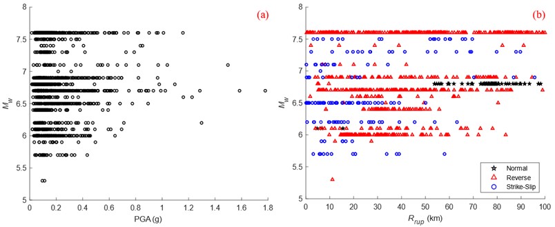
To implement this, the data is randomly split into an 80 % training set and a 20 % testing set. Bayesian regularization is employed to train the data. After several attempts, it was determined that the optimal regression performance was achieved when there were 10 hidden neurons. The obtained lateral displacement parameter sensitivity analysis model is shown in Fig. 2. According to the results in Fig. 2, it can be observed that both for the training set, validation set, and overall dataset, the predicted results have a correlation coefficient () of 0.94 or higher with the original target values. This indicates that predicted values of the model have a high level of reliability.
The sensitivity analysis was performed to assess how the 6 input features affect the predicted results of the model. Each input feature PGA, , , , FM and was multiplied by coefficient factors of 1.2 and 1.5 to create modified data for the second prediction using the model. The results of this second prediction were then compared with the initial predictions. Based on the changes in and RMSE values presented in Table 1, the correlation coefficients and root mean square error RMSE of the original data were used for comparison. From this analysis, it was observed that among the 6 input parameters, the lateral displacement value was most significantly influenced by , , and PGA, followed by FM, , and .
Fig. 2Training results of sensitivity analysis model for liquefaction drift parameters
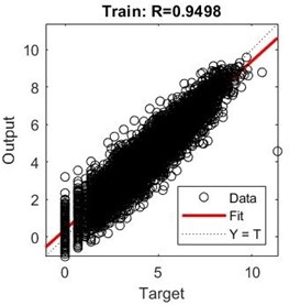
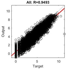
Table 1Input feature sensitivity analysis
Parameters | Coefficient of variation | RMSE | |
1.0 | 0.9493 | 0.6962 | |
PGA | 1.2 | 0.9454 | 0.9132 |
1.5 | 0.9304 | 1.3904 | |
1.2 | 0.9455 | 0.9476 | |
1.5 | 0.9248 | 1.8560 | |
1.2 | 0.8613 | 2.0743 | |
1.5 | 0.7256 | 5.7561 | |
1.2 | 0.9469 | 0.7238 | |
1.5 | 0.9347 | 0.8338 | |
FM | 1.2 | 0.9297 | 0.8237 |
1.5 | 0.8821 | 1.0501 | |
1.2 | 0.9468 | 0.7130 | |
1.5 | 0.9380 | 0.7704 |
4. The liquefaction lateral displacement prediction model and classical prediction model
Based on the original data and the sensitivity analysis results of the input features in Table 3, a neural network model was trained with the input features of , , and PGA. The Sigmoid function was chosen as the transfer function for the hidden layer. The dataset was randomly divided into 80 % training set and 20 % test set. Bayesian regularization was applied to train the data. After several trials, it was found that setting the number of hidden neurons to 7 yielded the best regression performance. The training results of the liquefaction lateral displacement prediction model are shown in Fig. 3. By comparing Fig. 3, it is evident that although reducing the number of input features in the liquefaction lateral displacement sensitivity analysis model has lowered the complexity of the model, it has also led to a slight decrease in prediction accuracy.
To objectively assess the reliability of the proposed liquefaction lateral displacement prediction model in this study, a comparison was made with three existing classical prediction models [10], [11] that use the same input variables (, , and PGA) and are based on the Newmark sliding block theory. To satisfy the constraints imposed by the literature [10], [11] and the prediction model proposed in this research, the ranges of , , and PGA are as follows, 5.5 ≤ ≤ 7.6, 0.01 ≤ ≤ 0.30 g, and 0.2 ≤ PGA ≤ 1.779 g, as shown in Fig. 4.
1. The Jibson 2007 model [10], referred to as J07:
2. The Rathje and Saygili 2009 model [11], abbreviated as RS09:
In Eq. (1-2), represents the lateral displacement, measured in cm.
Fig. 3Liquefaction side shift prediction model
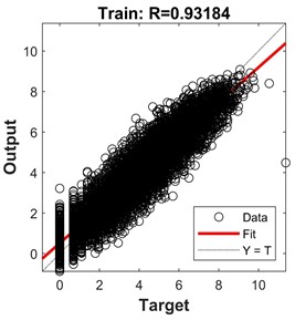
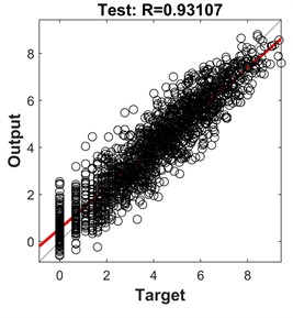
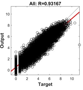
Fig. 4Comparison of the lateral spreading predictions model with the existing classical prediction models; a) variation with respect to Mw with ky= 0.15 g, PGA = 0.3 g; b) variation with respect to ky with Mw= 7.0, PGA = 0.3 g, c) variation with respect to PGA with Mw= 7.0, ky= 0.15 g
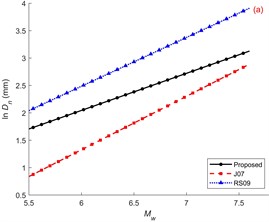
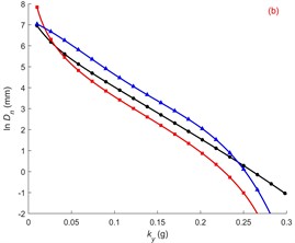
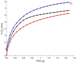
From Fig. 4(a), it can be observed that when the other seismic parameters are held constant, the lateral ground displacement increases with the increase in . This is because a larger indicates a greater amount of energy carried by the seismic waves, making the occurrence of liquefaction-prone conditions more likely in the seismic area. As a result, the lateral displacement also increases. Based on Fig. 4(b), it can be seen that when the other seismic parameters are constant, the lateral ground displacement decreases with an increase in . This can be understood as per the Newmark displacement calculation theory, which shows that the lateral displacement decreases with larger values of [6]. Additionally, a larger indicates a higher residual shear strength of the liquefied soil. Only when the combined shear force from seismic and gravitational actions exceeds the residual shear strength of the soil will it start to slide, leading to a decrease in lateral displacement. From Fig. 4(c), it can be observed that different PGA have varying effects on the lateral spreading displacement. However, overall, as the PGA increases, the lateral ground displacement also increases. This follows a similar pattern as the moment magnitude and is consistent with the Newmark displacement calculation theory [6]. Overall, the prediction model proposed in this study maintains good consistency with the existing classical models, while also aligning with theoretical analysis.
5. Conclusions
This study proposes a neural network-based liquefaction-induced lateral spreading prediction model based on the existing database and sensitivity analysis. The following conclusions are drawn.
1) The proposed prediction model demonstrates good consistency with existing classical models under the premise of agreement with theoretical analysis. This indicates that the developed model effectively captures the complex nonlinear relationships between input parameters and output parameters related to liquefaction-induced lateral spreading.
2) The sensitivity analysis results indicate that the lateral spreading value prediction is highly sensitive to moment magnitude, yield acceleration and peak ground acceleration. On the other hand, the impact of focal mechanism, the average shear wave velocity of the top 30 meters of soil, and rupture distance on lateral spreading is relatively small.
References
-
W. Zhang, X. Gu, L. Tang, Y. Yin, D. Liu, and Y. Zhang, “Application of machine learning, deep learning and optimization algorithms in geoengineering and geoscience: Comprehensive review and future challenge,” Gondwana Research, Vol. 109, pp. 1–17, Sep. 2022, https://doi.org/10.1016/j.gr.2022.03.015
-
Y. Yang, B. Yang, C. Su, and J. Ma, “Application of residual shear strength predicted by artificial neural network model for evaluating liquefaction-induced lateral spreading,” Advances in Civil Engineering, Vol. 2020, pp. 1–15, Aug. 2020, https://doi.org/10.1155/2020/8886781
-
S. Demir and E. K. Sahin, “Predicting occurrence of liquefaction-induced lateral spreading using gradient boosting algorithms integrated with particle swarm optimization: PSO-XGBoost, PSO-LightGBM, and PSO-CatBoost,” Acta Geotechnica, Vol. 18, No. 6, pp. 3403–3419, Jun. 2023, https://doi.org/10.1007/s11440-022-01777-1
-
M. Gade, P. S. Nayek, and J. Dhanya, “A new neural network-based prediction model for Newmark’s sliding displacements,” Bulletin of Engineering Geology and the Environment, Vol. 80, No. 1, pp. 385–397, Jan. 2021, https://doi.org/10.1007/s10064-020-01923-7
-
Z. Kaya, L. Latifoglu, E. Uncuoglu, A. Erol, and M. S. Keskin, “Predicting liquefaction-induced lateral spreading by using the multigene genetic programming (MGGP), multilayer perceptron (MLP), and random forest (RF) techniques,” Bulletin of Engineering Geology and the Environment, Vol. 82, No. 3, pp. 1–18, Mar. 2023, https://doi.org/10.1007/s10064-023-03103-9
-
N. M. Newmark, “Effects of earthquakes on dams and embankments,” Géotechnique, Vol. 15, No. 2, pp. 139–160, Jun. 1965, https://doi.org/10.1680/geot.1965.15.2.139
-
Y. Yang and E. Kavazanjian, “Newmark analysis of lateral spreading induced by liquefaction,” Journal of Earthquake Engineering, Vol. 26, No. 6, pp. 3034–3053, Apr. 2022, https://doi.org/10.1080/13632469.2020.1784316
-
T. D. Ancheta et al., “NGA-West2 database,” Earthquake Spectra, Vol. 30, No. 3, pp. 989–1005, Aug. 2014, https://doi.org/10.1193/070913eqs197m
-
W. Du and G. Wang, “A one-step Newmark displacement model for probabilistic seismic slope displacement hazard analysis,” Engineering Geology, Vol. 205, pp. 12–23, Apr. 2016, https://doi.org/10.1016/j.enggeo.2016.02.011
-
R. W. Jibson, “Regression models for estimating coseismic landslide displacement,” Engineering Geology, Vol. 91, No. 2-4, pp. 209–218, May 2007, https://doi.org/10.1016/j.enggeo.2007.01.013
-
E. M. Rathje and G. Saygili, “Probabilistic assessment of earthquake-induced sliding displacements of natural slopes,” Bulletin of the New Zealand Society for Earthquake Engineering, Vol. 42, No. 1, pp. 18–27, Mar. 2009, https://doi.org/10.5459/bnzsee.42.1.18-27
About this article

The authors have not disclosed any funding.
The datasets generated during and/or analyzed during the current study are available from the corresponding author on reasonable request.
The authors declare that they have no conflict of interest.
