Prediction of liquefaction time based on time-frequency distribution of seismic records

1. Introduction

The deformation of horizontally liquefied soil can be divided into three stages: small-magnitude seismic deformation before liquefaction, moderate-large deformation induced by seismic shaking after liquefaction, and permanent deformation after the earthquake [1]. Therefore, identifying the liquefaction time is important for evaluating the dynamic response of the site [2].

Several studies have been conducted to obtain the liquefaction time of the liquefied site, Yang and Kavazajian [3] used FLAC 2D to construct detailed profiles of five layers and obtained the liquefaction time of the site using the PM4sand constitutive model. Özener et al. [4] used power spectra, combined with Stockwell spectrograms to predict the liquefaction time. Zhang et al. [5] developed a liquefaction time prediction model by training a CNN using time-frequency spectral. These studies [3-5] have made significant contribution to the prediction of liquefaction time, while the method used in [3] requires highly detailed geotechnical investigation profile, the method proposed in [4] is relatively complicated, and the accuracy of the method in [5] depends on the number of the seismic motions used in the training of convolutional neural network.

In this research, based on the distribution of seismic records in the time and frequency domains, a new method for predicting liquefaction time is proposed. The real liquefaction time of the site is taken as the benchmark for comparison, and the accuracy of the proposed method as well as non-linear site response analysis method in determining liquefaction time are analyzed.

2. Site response analysis

The present study focuses on the analysis of the Treasure Island site during the 1989 Loma Prieta earthquake ($M_w=$ 6.9). This earthquake was characterized by various liquefaction phenomena, such as sand boiling and ground deformation [6]. Nonlinear analysis models of the site were established using DEEPSOIL and PLAXIS 2D. The deconvolution results of the bedrock seismic waves were used as inputs for the seismic waves. The liquefaction time of the site was determined based on the changes in effective stress.

2.1. Site liquefaction case

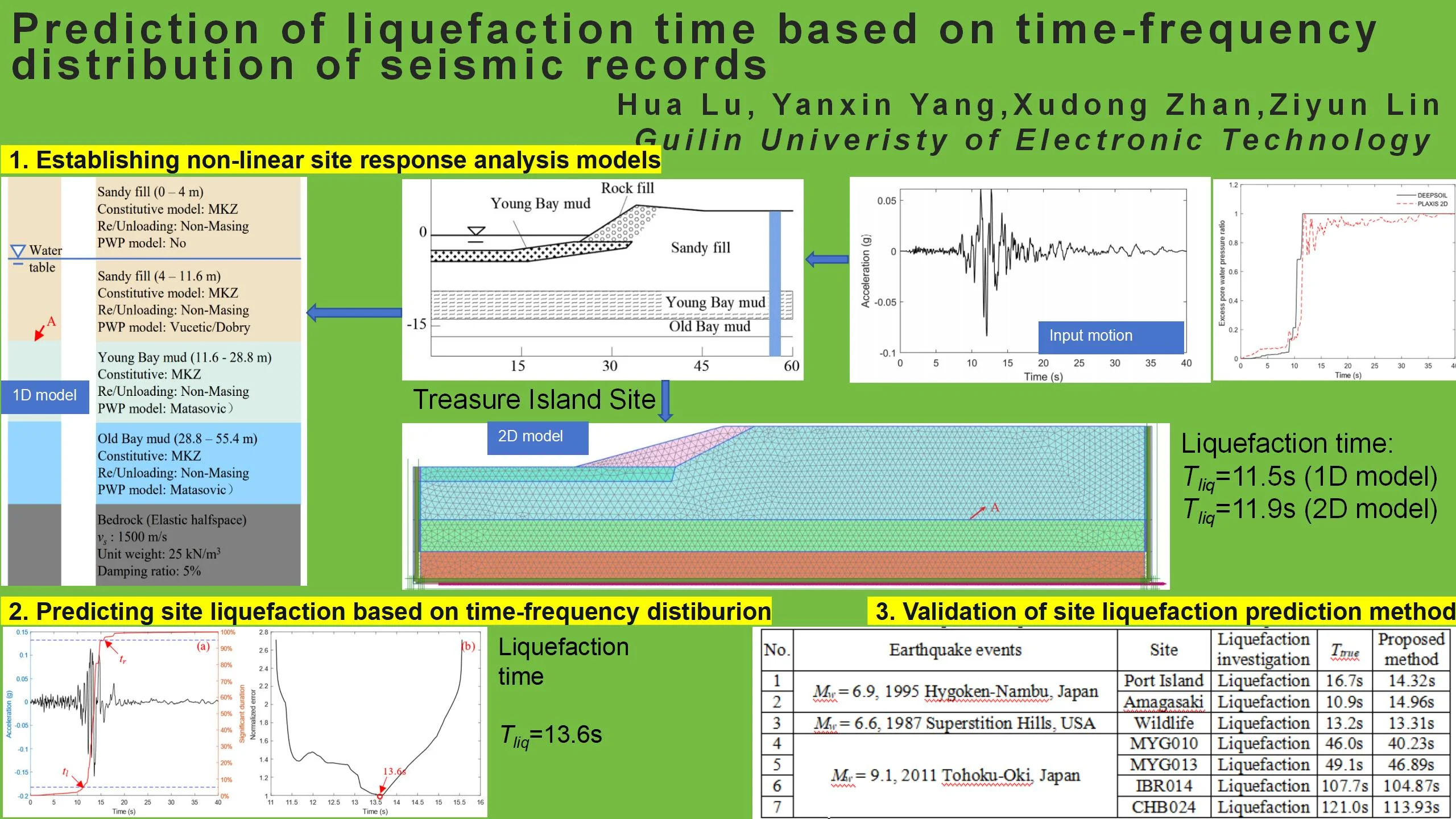
The soil profile and material parameters of the site are shown in Fig. 1 and Table 1 [7]. During the earthquake, bedrock motion was obtained near Treasure Island in Yerba Buena Island and deconvolution was performed on it. Based on the deconvolution analysis results, the horizontal ground motion records with rich energy content were selected using Arias intensity as inputs for DEEPSOIL and PLAXIS 2D analyses, as shown in Fig. 2.

Fig. 1The soil profile of Treasure Island [7]

Fig. 2Input earthquake records

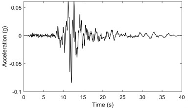
Table 1Basic size and style requirements [7]

Parameter	Rock fill	Sandy fill	Young Bay mud	Old Bay mud
Saturation (kN/m3)	28.1	18.4	16.5	19.2
dry density (kg/m3)	23	14.11	13.1	15.23
Cohesion (kPa)	1	1	5	5
Angle of internal friction (°)	36	33	25	25
Shear wave velocity (m/s)	500	152	186	336
Poisson’s ratio	0.3	0.3	0.45	0.45

DEEPSOIL is a one-dimensional site response analysis program developed by the University of Illinois, USA. It offers three types of site response analysis methods: linear, equivalent linear and non-linear [8]. According to reference [7], the sand fill material is identified as a liquefiable soil layer. To investigate the liquefaction time of the site, a soil column shown in Fig. 3 is constructed based on the blue column in Fig. 1. The stress-strain models for all layers are set as the MKZ model. The excess pore pressure model for the sand fill material below the groundwater level adopts the Vucetic/Dobry model, while the Holocene and Pleistocene Bay Mud layers use the Matasovic excess pore pressure model. The bedrock is modeled as an elastic half-space with $V_s$ of 1500 m/s, a unit weight of 25 kN/m³, and a damping ratio of 5 %. The dynamic shear modulus and damping ratio are determined based on experimental results from reference [10]. The monitoring point for excess pore pressure is located at point A, at an elevation of –11.6 m, at the bottom of the sand fill material layer.

PLAXIS 2D is selected as the software for two-dimensional non-linear site response analysis. Based on the soil parameters of Treasure Island shown in Fig. 1 and Table 1, and referring to the research findings from reference [11], the following parameters are adopted. The Mohr-Coulomb model is used to generate initial stresses in the soil layers based on the available data. The UBC3D-PLM sand liquefaction model is applied to the liquefiable soil layer, while the remaining non-liquefiable soil layers are modeled using small-strain soil hardening models. The UBC3D-PLM model includes several key parameters, peak friction angle (${\phi }_p$), friction angle at constant volume (${\phi }_{cv}$), effective cohesion ($c$) and the normalized SPT blow count [($N_1$)₆₀]. Among them, the value of ($N_1$)₆₀ is determined through back-analysis based on Eq. (1) [12]. For Sandy fill, ${\phi }_p=$ 31.29°, ${\phi }_{cv}=$ 30.45°, $c=$ 1kPa and ($N_1$)₆₀ = 8.45:

1

${\phi }^{\mathrm{\text{'}}}=\sqrt{20\mathrm{*}(N_1{)}_{60}}+20.$

Fig. 3The parameters of DEEPSOIL soil column model

To ensure that the shear strength at the lateral boundaries is not completely lost, as this could lead to excessive deformations, a Mohr-Coulomb constitutive model is applied with a 1-meter-wide drained boundary at the lateral boundaries. Additionally, to mitigate the influence of high-frequency components in the seismic motion, the Rayleigh damping method proposed in reference [13] is implemented. Considering the propagation theory of seismic waves in an elastic half-space, a horizontal displacement component of 0.5 meters is assigned.

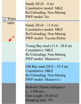
Based on the above considerations, a numerical model is established with 6651 elements and 54510 nodes. The grid of model is depicted in Fig. 4.

Fig. 4Finite element analysis model

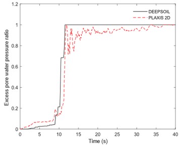
The input for DEEPSOIL and PLAXIS 2D is the bedrock seismic wave shown in Fig. 2, which is used for non-linear site response analysis. The excess pore water pressure time history at location A is obtained and depicted in Fig. 5. The black solid line represents the calculation results from DEEPSOIL, while the red dashed line represents the results from PLAXIS 2D. The liquefaction time predicted by DEEPSOIL is 11.5 s, while the liquefaction time predicted by PLAXIS 2D is 11.9 s.

3. Prediction method of site liquefaction time

Earthquake signals are non-stationary time-domain signals, and the frequency components of the ground motion will change due to liquefaction. If the phase shift of the motions could be captured, then the corresponding liquefaction time could be obtained. Thus, this paper proposed a method for predicting the site liquefaction time as follows.

1. Select a seismic record with abundant energy in the horizontal direction based on the Arias intensity. Apply the Hilbert-Huang Transform (HHT) to process the ground acceleration time history. From the Hilbert spectrum, extract the excellent frequency curve by identifying the frequency corresponding to the maximum energy at each time instant. The specific physical interpretation of the excellent frequency is discussed in detail in reference [14].

2. Use the 90 % significant duration [15] to capture the excellent frequency time history within the corresponding time interval. Define the average frequency on the left and right beam sections at any given time as the step function, represented by $f_l$ and $f_r$.

Fig. 5The excess pore water pressure ratio time history

3. Define the difference between the excellent frequency and the step function at any given time as the error function $E\left(t\right)$, as shown in Eq. (2). This error function effectively identifies the moments of rapid frequency change in the acceleration-time-frequency curve of the seismic record:

where, $f_m$ represents the average frequency at time $t$, $f$ represents the excellent frequency at time $t$, and $t_l$ and $t_r$ represent the start and end times, respectively, of the time interval within which the 90 % significant duration occurs.

4. Normalize the error function, and the time corresponding to $E\left(t\right)=$ 1 is considered as the estimated liquefaction time for the site.

3.1. Case analysis of Treasure Island

The proposed method was applied to process the ground seismic records monitored at the Treasure Island station during the 1989 Loma Prieta earthquake. The 90 % significant duration of the seismic record is shown in Fig. 6(a), from the PEER-NGA-West2 database [16]. Additionally, the corresponding normalized error function time history is shown in Fig. 6(b).

Fig. 6a) Treasure Island acceleration time history [16], b) error function curve

The minimum value of the normalized error function corresponds to the estimated liquefaction time. From Fig. 6(b), the normalized error function occurs at approximately 13.6 s, indicating that liquefaction likely occurred at parts of the Treasure Island site at around 13.6 s.

4. Validation of time-frequency site liquefaction prediction method

Based on the seven liquefaction sites with known liquefaction times from the 1995 Hyogoken-Nambu earthquake in Japan, the 1987 Superstition Hills earthquake in the United States, and the 2011 Tohoku-Oki earthquake in Japan, this paper further validates the reliability of the method for determining liquefaction times. To assess the correlation and reliability between the predicted liquefaction times and the actual liquefaction trigger times, the coefficient of determination ($R^2$), as shown in Eq. (3), can be introduced. Based on a total of 7 cases in Table 2 and Treasure Island site, the calculated $R^2$ for the method is 0.99. This suggests that the proposed method exhibits a high level of reliability in predicting liquefaction time for different seismic events and sites:

where, $T_{true}$ represents the true liquefaction time, $T_{pre}$ represents the predicted liquefaction time, and $T_{mean}$ represents the mean of the predicted liquefaction times.

5. Conclusions

The present study proposes a new method for predicting liquefaction initiation time based on the time-frequency characteristics of ground acceleration. The defined step function and error function in this research effectively identifies the moments of rapid frequency changes in the ground seismic records, enabling the prediction of liquefaction initiation time. A $R^2=$ 0.99 during the validation for 8 documented liquefaction sites associated with 4 seismic events indicates this method is reliable.

It should be noted that the proposed method only utilizes horizontal ground motion records. The inclusion of vertical ground motion records in the prediction of liquefaction initiation time may potentially improve the accuracy of the results.