The computational method of substructure’s frequency response function in transfer path analysis

1. Introduction

At present, characteristics of Noise, Vibration and Harshness (NVH) have become one of the key factors in the design of vehicles. A number of methods have been established to solve NVH problems, including Computer Aided Engineering (CAE) technology and excitation source identification etc. [1-3]. Transfer Path Analysis (TPA) methods [4], included Classic TPA (CTPA) [5], Operational TPA (OTPA) [6] and Operational Path Analysis with eXogeneous Inputs (OPAX) [7] and so forth, have been widely applied in engineering practice in the application process of identifying excitation source. The key points for TPA method are the measurement of the FRF and the identification of the operating load. However, the active substructure needs to be disassembled in the CTPA method, measured the FRF of the passive substructure after physical decoupling, produced some bad effects, including the long disassembly time and could be changed the boundary conditions etc. [8]. The characteristic of the OTPA method is the transmissibility replacement of the FRF in the OTPA method with the relationship between different responses, while it is different from other TPA methods based on the relationship between load and response. Since the transmissibility with various operational conditions, it is not an inherent property of the vehicle structure. Although the active substructure does not need to be disassembled with the method, while it caused some disadvantages such as cross coupling of the excitation sources, incorrect estimation of the transmissibility function and omission of the transfer path etc. [9, 10]. The OPAX method is used to measure FRF by reciprocal principle and identify load by parametric load model, which has a good compromise between accuracy and engineering efficiency. However, some measurement locations cannot be achieved by the reciprocal measurements, such as the steering wheel and instrument panel, therefore, the active substructure must still be disassembled [11-13]. In order to solve the problems of the CTPA, OTPA and OPAX methods, the FRF of substructure which cannot be measured by the reciprocity principle is obtained by the computational method of the substructure’s FRF proposed in this paper without disassembling the active substructure. The FRF of substructure and the dynamic mount stiffness are derived from the FRF of the multi-degree-of-freedom coupled vibration system, therefore, without obtaining the dynamic mount stiffness from the vibration table.

On the other hand, the coupling problem of the linking components is solved by the computational method of the substructure’s FRF without disassembling the active substructure compared with the TPA method. Okubo N. [14] proposed an analysis method for substructure. Under the known of some substructure characteristics premise, the dynamic characteristics of unknown substructure can be derived by known substructure not from the system level. Keersmaekers L. [15] proposed a Link-Preserving, Decoupling Method (LPD method). The FRF of coupled linking components was derived on the consistency of coupled stiffness matrix characteristics of linking components, but the internal FRF of passive substructure was not deduced. Wang Z. [16] put forward a decoupling transfer function prediction method based on in-situ transfer function, which was verified by LPD, but the verification process was only carried out on the vehicle model. Xuhui Liao [17] came up with the method that simplified the complex mathematical derivation through the elementary row change of matrix based on the same number of coupled degrees of freedom. The coupled dynamic stiffness of the linking components was not deduced, and it was not tested and verified in the coupled vibration system of real vehicle.

Based on the dynamic equation of the multi-degree-of-freedom coupled vibration system, the FRF of the substructure and the dynamic stiffness of the linking components are derived from the FRF of the system level. Under the assumption of linear and time-invariant, the real vehicle is simplified into a multi-degree-of-freedom coupled vibration system with “engine-mount-body” as the transfer path. The computational method of the substructure’s FRF based on the FRF of system obtained by the hammering test proposed in this paper is used to derive the FRF of substructure and dynamic mount stiffness from the FRF of system. Combining the dynamic mount stiffness with the vibration acceleration of the active and passive sides of the mount, the operating load is identified by the mount-stiffness method of the transfer path. Based on the relationship between load and response, the FRF of substructure is incorporated with operating load to analyze the contribution of real vehicle transfer path.

2. Multi-degree-of-freedom coupled vibration system

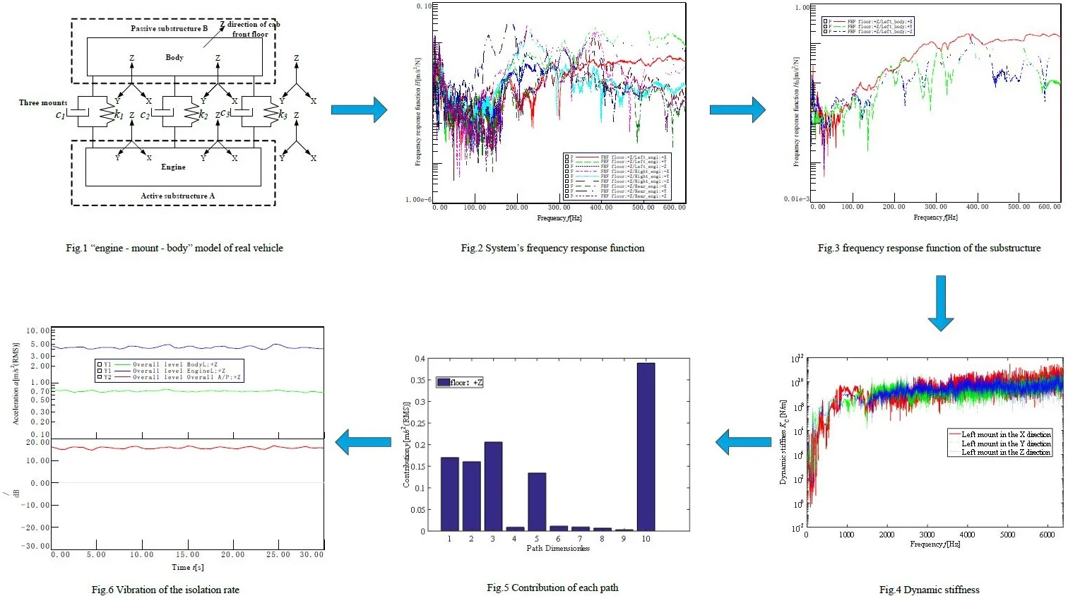
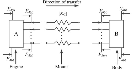
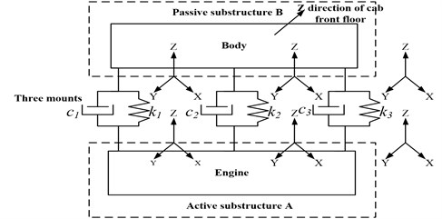
As the coupled problem of the linking components between the two substructures, the excitation source needs to be disassembled to achieve decoupling based on the traditional transfer path analysis. However, the excitation source is not disassembled in the transfer path analysis based on the computational method of the substructure’s FRF. The vehicle system is divided into two independent substructures connected by elastic and damping linking components to form the multi-degree-of-freedom coupled vibration system. For example, the coupled vibration system of a vehicle is simplified into an analysis model of “engine (active substructure A) – mount (linking components) – body (passive substructure B)”. The simplified multi-degree-of-freedom coupled vibration system is shown in Fig. 1.

The relationship between the input and output of the system is described in Fig. 1. Theoretically, the expression of a system with two substructures in the frequency domain is:

where, ${\mathbf{X}}_A\left(j\omega \right)$ and ${\mathbf{X}}_B\left(j\omega \right)$ represent the response vectors of active substructure A and passive substructure B respectively, ${\mathbf{F}}_A\left(j\omega \right)$ and ${\mathbf{F}}_B\left(j\omega \right)$ represent the excitation force vectors acting on active substructure A and passive substructure B correspondingly, ${\mathbf{H}}_{xy}\left(j\omega \right)$ ($x=A$ or $B$, $y=A$ or $B$) denotes the FRF matrix, for example, ${\mathbf{H}}_{BA}\left(j\omega \right)$ denotes the FRF matrix between the excitation force vector ${\mathbf{F}}_A\left(j\omega \right)$ and the response vector ${\mathbf{X}}_B\left(j\omega \right)$. The Eq. (1) can be further amplified for the following as:

For the easier to write, the frequency $\omega$ is omitted in the formula (same as below). Superscripts $i$ and $c$ signify the internal degrees of freedom of the substructure and the coupling degrees of freedom of the linking components, respectively. ${\mathbf{X}}_A^i$, ${\mathbf{X}}_A^c$, ${\mathbf{X}}_B^i$ and ${\mathbf{X}}_B^c$ signify the response vectors of the excitation force vector ${\mathbf{F}}_A^i$, ${\mathbf{F}}_A^c$, ${\mathbf{F}}_B^i$ and ${\mathbf{F}}_B^c$ applied to the active and passive substructures respectively, ${\mathbf{H}}_{xy}^{MN}$ ($x=A$ or $B$, $y=A$ or $B$, $M=i$ or $c$, $N=i$ or $c$) signify the FRF matrix, for instance, ${\mathbf{H}}_{BA}^{ic}$ signify the FRF matrix between the excitation force vector ${\mathbf{F}}_A^c$ and the response vector ${\mathbf{X}}_{\mathrm{B}}^i$.

Fig. 1Multiple-degree-of-freedom coupled vibration system

3. The foundational formula of substructure’s FRF and dynamic mount stiffness

4. Acquisition of measured data in transfer path analysis

4.2. Collection of operating data

Seven 3-direction acceleration sensors were installed on target location and each of the three mounts’ active and passive sides. The arrangement of measurement locations is shown in Fig. 2. The operating data was collected under idling speed of 800 r/min, including $X$, $Y$ and $Z$ direction vibration acceleration signals of active and passive sides of three mounts. The measured acceleration data in the $Z$ direction of the three mounts’ active and passive sides are shown in Fig. 3-5.

Fig. 2The arrangement of measuring locations

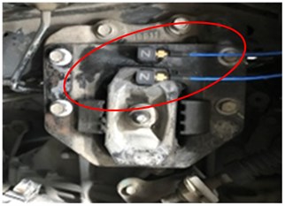
a) Left mount of engine

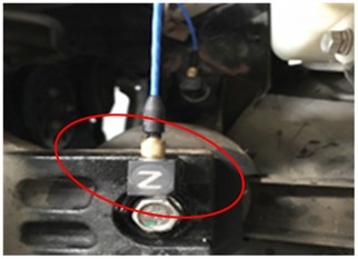
b) Right mount of engine

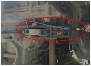
c) Rear mount of engine

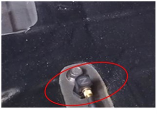
d) Target location

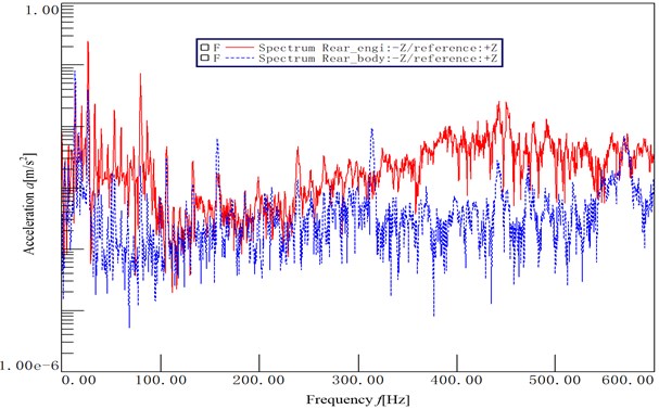
According to Eq. (21), when the mount-stiffness method was used to identify the load, the acceleration’s frequency-domain signals of active and passive sides of the three mounts were required, reserving the phase information of the data. Therefore, the collected time-domain signals were transformed into frequency-domain signals ${\mathbf{a}}_{aj}\left(\omega \right)$ and ${\mathbf{a}}_{pj}\left(\omega \right)$ by Fourier transform. The acceleration’s frequency-domain signals of the active and passive sides of the three mounts in the $Z$ direction are shown in Figs. 6-8.

Fig. 3Time-domain signals of active and passive sides of the left mount in Z direction

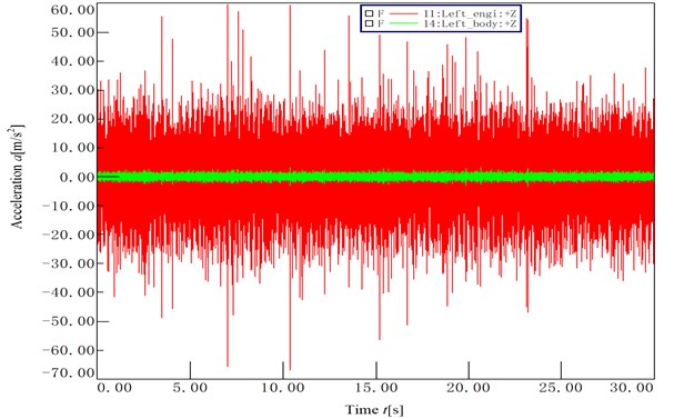
Fig. 4Time-domain signals of active and passive sides of the right mount in Z direction

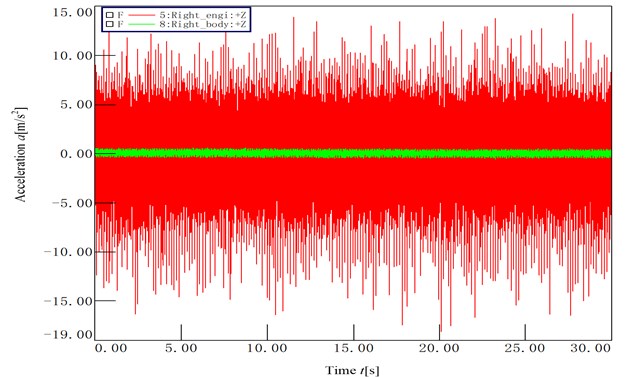
Fig. 5Time-domain signals of active and passive sides of the rear mount in Z direction

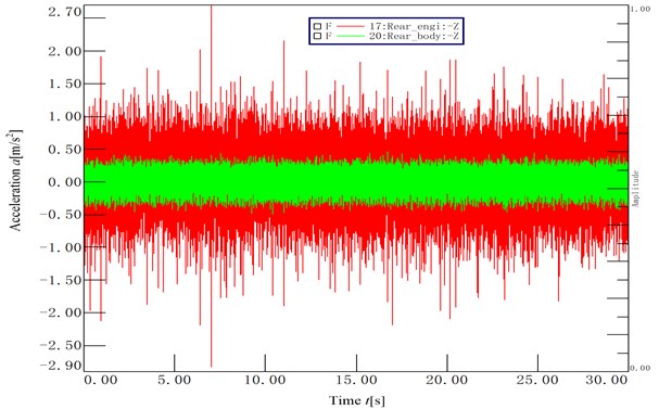
Fig. 6Frequency-domain signals of active and passive sides of the left mount in Z direction

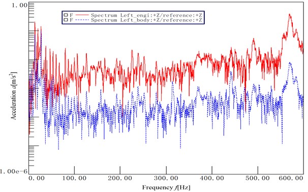
Fig. 7Frequency-domain signals of active and passive sides of the right mount in Z direction

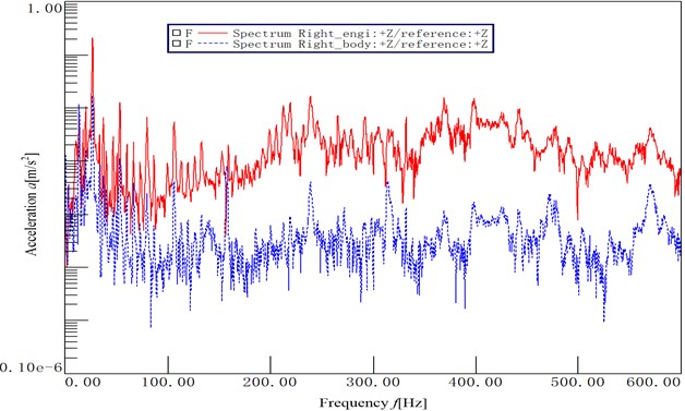
Fig. 8Frequency-domain signals of active and passive sides of the rear mount in Z direction

4.3. Measurement of system’s frequency response function

The measurement of the FRF of system obtained from hammering test in the process, the acceleration sensors of target location and mount’s active and passive sides were retained. In order to reduce the calculation complexity of the computational method of the substructure’s FRF, we take only one target location, $Z$-direction of the front floor of the cab, to simplify the matrix operation. The multi-degree-of-freedom coupled vibration system of “engine-mount-body” forms a model that inputs nine singles and outputs just one single, as shown in Fig. 9.

Fig. 9“Engine-mount-body” model of real vehicle

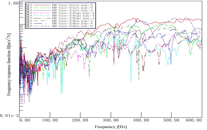
The hammering test was used to get the FRF of system of the Eq. (7) by hammering in the $X$, $Y$ and $Z$ directions of the active and passive sides of each mount, respectively, produced the hammering signal as the excitation signal, and simultaneously collecting the response signal from the acceleration sensor at the active and passive sides of the mount and the target location. Therefore, we get 9×9 size of system’s FRF matrix ${\mathbf{H}}_{AA}^{cc}$ in the mount’s active side, 9×9 size of system’s FRF matrix ${\mathbf{H}}_{BB}^{cc}$ in mount’s passive side, 9×9 size of system’s FRF matrix ${\mathbf{H}}_{BA}^{cc}$ from mount’s active side to mount’s passive side, 1×9 size of system’s FRF matrix ${\mathbf{H}}_{BB}^{ic}$ from mount’s passive side to target location, 1×9 size of system’s FRF matrix ${\mathbf{H}}_{BA}^{ic}$ from mount’s active side to target location and 1×1 size of system’s FRF matrix ${\mathbf{H}}_{BB}^{ii}$ in target location. some of the system’s FRF curves from the $X$, $Y$ and $Z$ directions of the three mounts’ active and passive side to the target location, are shown in Fig. 10 and Fig. 11.

Fig. 10The system’s FRF from the active side of mounts to the target location

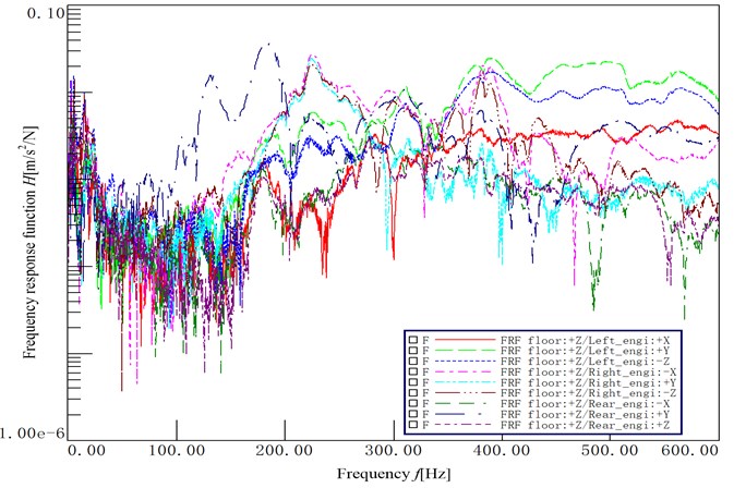
Fig. 11The system’s FRF from the passive side of mounts to the target location

4.4. The substructure’s FRF and the dynamic mount stiffness

The FRF of the substructure and the dynamic mount stiffness can be calculated through the derivation of the basic equation in Section 3 and the measured FRF of the system in Section 4.3. Concretely, the FRF ${\mathbf{H}}_{d,b}^{ic}$ from the coupling degrees of freedom of the passive side of the mount to the internal degrees of freedom of substructure B is calculated by Eqs. (7) and (9). When using MATLAB to code the algorithm, the FRF of system is a function of frequency causing the fact that the two-dimensional matrix cannot be presented, so the three-dimensional matrix expression was adopted. The FRF of the substructure from the $X$, $Y$ and $Z$ directions of the three mounts’ passive sides to the target point, namely, the uncoupled FRF from the operating load to the target point, are as shown in Figs. 12-14.

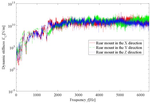
According to Eq. (18), the dynamic stiffness in the $X$, $Y$ and $Z$ directions of the three mounts can be calculated respectively, as shown in Figs. 15-17.

Fig. 12The FRF of the substructure from the passive side of the left mount to the target location in Z direction

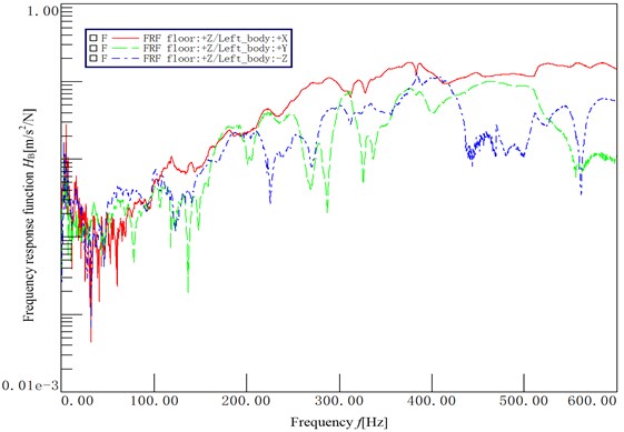
Fig. 13The FRF of the substructure from the passive side of the right mount to the target location in Z direction

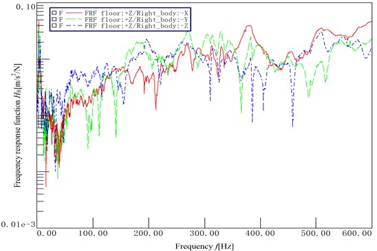
Fig. 14The FRF of the substructure from the passive side of the rear mount to the target location in Z direction

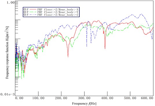
Fig. 15The dynamic stiffness in the X, Y and Z directions of the left mount

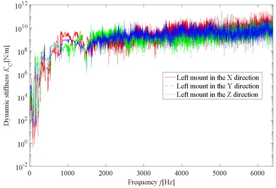
Fig. 16The dynamic stiffness in the X, Y and Z directions of the right mount

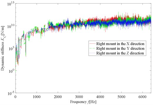
Fig. 17The dynamic stiffness in the X, Y and Z directions of the rear mount

5. Contribution analysis of real vehicle transfer path

According to the basic theory of transfer path analysis, it was necessary to identify the operating load for contribution analysis. The operating load can be calculated by substituting the dynamic mount stiffness calculated in Section 4.4 and the acceleration data in frequency-domain collected in Section 4.2 into Eq. (21). The contribution of each transfer path to the target location can be analyzed by substituting the operating load and the FRF of substructure calculated in Section 4.4 into Eq. (20).

Path 1 to Path 3 denotes respectively the path contribution of left mount in $X$, $Y$ and $Z$ directions, Path 4 to Path 6 denotes respectively the path contribution of right mount in $X$, $Y$ and $Z$ directions, Path 7 to Path 9 denotes respectively the path contribution of rear mount in $X$, $Y$ and $Z$ directions, and Path 10 denotes the total contribution of each path to target location.

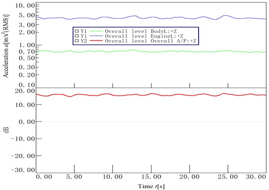
It can be seen from Fig. 18 that the contribution of the left mount $Z$ direction to the target location is the most dominant. The vibration isolation rate in the $Z$-direction of the left mount was analyzed by using the Overall data of the active and passive sides of the left mount obtained through operating data, which can be expressed in the form of dB:

where, $T_{dB}$ is the vibration isolation rate of the mount, ${\mathbf{a}}_a$ is the vibration acceleration of the mount’s active side, and ${\mathbf{a}}_p$ is the vibration acceleration of the mount’s passive side. When the vibration isolation ratio $T_{dB}$ > 20 dB, the mount has good vibration isolation effect, meeting the vibration isolation requirements. When the vibration isolation ratio $T_{dB}$ < 20 dB, the mount has poor vibration isolation effect.

Fig. 18The contribution of each path

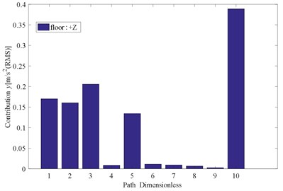
Fig. 19 shows the vibration isolation rate of left mount in the $Z$ direction. As seen from the figure, the vibration isolation rate of left mount in the $Z$ direction is less than 20 dB, so the vibration isolation effect of left mount in the $Z$ direction is poor. It is shown that the left mount in the $Z$ direction is the main contribution path of the target location, which further verify the accuracy and effectiveness of the computational method of the substructure’s FRF in the transfer path analysis.

Fig. 19Vibration isolation rate of left mount in Z direction

6. Conclusions

1) The computational method of the substructure’s FRF was proposed on the basis of the multi-degree-of-freedom coupled vibration system of transfer path, and the core of the method is that basic formulas of the FRF of substructure and the dynamic mount stiffness was derived from the FRF of system. Thus, the essential relationship among the FRF of system, the FRF of substructure and the dynamic mount stiffness were obtained in the process.

2) Taking the “engine-mount-body” of a real vehicle as the transfer path, the FRF of the system was obtained by hammering test without disassembling the excitation source combined with the method proposed in Section 3, the FRF of passive substructure B (the uncoupled FRF) required for real vehicle transfer path analysis was calculated and the dynamic stiffness of the mount can also be obtained from the system level. The advantage of this method was that it can avoid the time-consuming and laborious problem of disassembling the excitation source.

3) Combined with the acceleration data in frequency-domain under idling speed of 800 r/min of the real vehicle and dynamic mount stiffness, the operating load of the real vehicle was identified on the basis of the mount-stiffness method. Combining the operating load and the FRF of passive substructure B, the contribution of each path is analyzed to find the path with the largest contribution to the target location. The accuracy and effectiveness of the computational method of the substructure’s FRF were verified by the calculation results of the vibration isolation rate, which provided theoretical support for the study of dynamic characteristics of substructure and the linking components.