Modeling method of failure dependent system based on time varying copula function

Xing, Mengli; Xu, Dan; He, Jiaolan

doi:10.21595/vp.2017.19172

Vibroengineering Procedia

Browse Procedia

Published: 21 October 2017

Check for updates

Modeling method of failure dependent system based on time varying copula function

Mengli Xing¹

Dan Xu²

Jiaolan He³

^{1, 2, 3}School of Reliability and Systems Engineering, Beihang University, Beijing, China

Corresponding Author:

Mengli Xing

Cite the article Download PDF

Downloads 1469

Abstract

This paper aims at solving the dynamic correlation of the complex dependence system with multiple failures. A correlation model and parameter estimation method based on time-varying copula function are proposed to solve the joint distribution between the interaction mechanism. In particular, three types of definition method for the time-varying copulas’ parameters are introduced. Finally, a comparative study and applicability analysis are performed to validate our proposed method.

1. Introduction

In reality, there are several failure modes for a complex system with multiple components and complicated structure when subjected to the diverse running environment. In general, the relationship between the failure modes will change with the use of equipment. According to the classification of the failure behavior modeling, this correlation can be reflected by the failure variable of each component or the performance parameters of the system. In this paper, based on the performance parameters of the system, we proposed a modeling method to study the correlation between the dynamic failure model.

Reviewing previous studies, we can find that the research on the failure dependent system mainly concentrate on two aspects: one aspect is based on the components to establish the logical model of the system and parameter model, and specific parameters of common cause are introduced to quantify the influence of the common cause failure [1-4]. the other aspect is typical failure modeling approach based on the observation data of performance parameters. It’s noted that there often exists dependent relationship between the performance parameters of the system due to the common cause failure, therefore some scholars utilized stochastic process or other statistical method to model the distribution of performance parameters, and finally copula function is introduced to establish the reliability model of the system [5-8]. Copula can be divided into two categories according to whether its parameters are time-varying or not: type I and type II, that is, static copula and dynamic copula. For the former, its parameter is a constant time-independent value that stands for the constant dependency structure between variables, which is widely used in the reliability modeling of joint distribution [9, 10]. However, considering the dependence between variables fluctuated due to the change of the external environment, time-varying copula model is proposed to study the dependent relationship between two or more variables over time. The key to construct the time-varying copula model is to give the evolution equation of parameters of the copula function. However, there is no point in forcing a variable to follow a certain process without knowing the meaning and influence of the parameter.

According to the different specification of time-varying parameters, Patton [11] proposed a similar ARMA (1, 10) process to describe the related parameters of two normal copula function; Manner and Hafner [12] proposed the stochastic autoregressive copula model(SCAR), where the time-varying copula parameter is a transformation of a latent Gaussian AR(1) process; Creal et al. [13] presented a generalized autoregressive score (GAS) model, which not only assumes an latent process for the parameter, but also utilized the weighted score of the underlying model to drive the latent process. In addition, DCC model [16] and semiparametric approach [17] were also introduced to the definition for dynamic copula parameters. The methods above have one similarity, that is they all used the feature that there is the one-to-one relationship between the parameters of copula and correlation coefficient. Therefore, once the correlation coefficient of copula function is determined, the corresponding evolution equation of copula function parameter will be determined. However, it’s noticed that all these time-varying copula model are derived from the financial field, and are particularly scarce in the field of reliability. It’s worth noting that the latest application research in reliability is still stuck in bivariate time-varying copula [18], and its time-varying parameter definition method is still based on the theory presented by Patton in 2006, without new breakthrough. Therefore, in order to conduct the reliability modeling method for the complex system with dependent multiple variables, especially considering the time-varying nonlinear correlation between failure modes, a proper modeling method needs to be further studied.

2. Multivariate coupling modeling method based on time varying copula

Copula theory provides a theoretical basis for the construction of coupled multivariate model. As the function connecting the marginal distribution and the random variable, copula can not only describe the correlation between random variables, but also reflect the dependency structure. Based on copula function, the construction of the multivariable joint distribution model is mainly divided into two steps: one step is to determine the marginal distribution model of each variable; the other step is to select the most appropriate copula function to fuse marginal distribution according to the characteristics of different copula function.

2.1. Selection of the marginal distribution

The selection of the marginal distribution model can be considered from two aspects:

i) Acquisition of the marginal distribution based on statistical model.

Take degradation modeling as an example: According to the characteristic of the degradation path, we can use degradation data for statistical inference to obtain the degradation model. In the process, different statistical model can be introduced, then the corresponding marginal distribution form can be determined. However, the hypothesis test of distribution is necessary when using this method

ii) Acquisition of marginal distribution based on empirical model.

When the specific form of the distribution is unknown, the empirical distribution model can be used to simulate the distribution function. At this time, by empirical distribution, the marginal distribution can be expressed as:

1

{\hat{F}}_{X} (x) = \frac{1}{n} \sum_{i = 1}^{n} 1 \{X_{i} < x\} .

After determining the marginal distribution of each variable, we can choose different copula forms to establish the coupling model according to the different feature of copula function.

2.2. The selection of time-varying copula

In this paper, we focus on three types of time-varying parameter definition methods: the generalized autoregressive score model (GAS model), the autoregressive conditional parameter model (ACP) based on Patton’s theory, and the SCAR model, which is introduced to study their modeling method and application in the field of reliability for multiple failure dependent systems.

Let $y_{t} = (y_{1, t}, \dots y_{p, t}) t = 1,2, . . . T$ denotes a sequence of $T \times p$ dimensional failure variable, according to Sklar’s theorem, there exists copula function:

2

G (y_{1, t}, \dots y_{p, t}) = C (F_{1, t}, . . . F_{p, t}),

where $F_{i, t}$ is the distribution of the $i$ th failure variable. We can define $u_{i, t} = F_{i, t}$ , then assume that arbitrary time series of distribution of bivariate failure variables follows the distribution $(u_{i, t}, u_{j, t}) ~ C (., .; θ_{t})$ , where $θ_{t}$ is the time-varying parameter of copula, and generally can be expressed by $θ_{t} = Λ (λ_{t})$ . It has been found that there is a one-to-one transition between copulas’ parameter and Kendall’s coefficient $τ$ , then $θ_{t} = r (τ_{t})$ . As mentioned above, the evolution equation of the correlation coefficient $τ$ will be given based on the GAS (1, 1) model, the SCAR model and the Patton’s model, respectively.

In GAS (1, 1) model, we have:

3

λ_{t} = ω + β λ_{t - 1} + α s_{t - 1} .

In Eq. (3), $s_{t} = S_{t} \nabla_{t}$ is the scaled score vector corresponding to the log-likelihood function, where $\nabla_{t}$ can be expressed as:

4

\nabla_{t} = \frac{\partial l n c (u_{i, t}, u_{j, t}; ϖ, R_{t - 1})}{\partial θ_{t}},

where $ϖ = (ω, β, α)$ , the scaling matrix $S_{t}$ is the square root matrix of the inverse matrix of the information matrix, which can be defined as:

5

S_{t} = J_{t | t - 1}, \begin{array}{l} J_{t | t - 1}^{'} J_{t | t - 1} = I_{t | t - 1}^{- 1} \end{array},

where $I_{t | t - 1} = E_{t - 1} [\nabla_{t} {\nabla^{'}}_{t}]$ is the information matrix.

As Patton’s theory, time-varying Joe-Clayton copula model and normal copula model were presented, where the time-varying parameter $ρ$ in the normal copula function can be described as a similar ARMA (1, 10) process, then we have:

6

ρ_{t} = Λ (ω + β ρ_{t - 1} + α \frac{1}{10} \sum_{i = 1}^{10} Φ^{- 1} (u_{t - i}) Φ^{- 1} (v_{t - i})) .

In this paper, Patton's theory is extended and summarized. The dynamic Clayton copula function and the dynamic Gumbel copula function are introduced to measure the asymmetric dependence of multiple variables. Since the Clayton copula is more sensitive to the change of the lower tail, and the Gumbel copula is more sensitive to the change of the upper tail, so we use the Clayton copula to describe the stronger relationship in lower tail, while the Gumbel copula is used to describe the stronger relationship in upper tail. For these two copula functions, the equation is defined as follows:

7

θ_{t} = Λ (ω + β θ_{t - 1} + α \frac{1}{m} \sum_{i = 0}^{m - 1} |u_{1, t - i} - u_{2, t - i}|) .

In SCAR function, its parameter is driven by an independent random process. Generally, the time-varying parameters can be denoted as $θ_{t} = Λ (λ_{t})$ , where the underlying process ${\{λ_{t}\}}_{t = 1}^{T}$ is assumed to obey a Gaussian autoregressive process as:

8

λ_{t} = ω + β λ_{t - 1} + α_{η} η_{t},

where $η_{t}$ is the i.i.d. standard normal distribution, and $|β| < 1$ ensures the stationarity of $λ_{t}$ . In the estimation of the parameters, the solution of the time-varying coefficients cannot be directly carried out restricted that $λ_{t}$ is a hidden process. Under such circumstance, the likelihood function of the time-varying parameter $ϖ$ can be achieved through the integration of the hidden process, namely:

9

L (ω; u_{i}, u_{j}) = \int f (u_{i}, u_{j}, Λ; ω) d Λ .

To solve this multidimensional integral, the numerical solution can be obtained by Monte Carlo integral based on the effective importance sampling (EIS) [15] method.

3. Case study

In this paper, electronic smart meter is selected as a case study, where a comprehensive environmental test with two stress (temperature: 70 °C and humidity: 95 %) is conducted for the smart meter. The smart meter is a product with many failure dependent components and the failure correlation can be characterized by the output parameters, so we use the data of output performance parameters collected from the test and failure characterization to study the dynamic modeling method for the system failure. In the test, the data of two key characteristics performance parameters is obtained, and the corresponding trajectories of test data are shown in Fig. 1.

Fig. 1Observation data of the key performance characteristics of electric smart meters

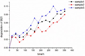
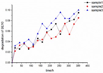
Through the analysis of the observation of the characteristic performance parameter, we can find that the data presents fluctuation. At the same time, the observation data of the performance characteristic at the time $t$ is not a fixed value, but follows a distribution due to the influence of the sample dispersion. Consider that the specific distribution is unknowable and the assumed distribution type may cause errors to the modeling results, empirical cumulative distribution method is introduced to derive the value of the distribution. Finally, $F_{i, t}$ , the distribution of $i$ th performance characteristic at each time t is computed.

Fig. 2The curve of time-varying parameter θt based on Patton’s model

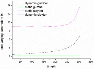
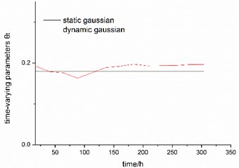
Having obtained the distribution function of the performance characteristic, three types of time varying copulas: Clayton copula, Gumbel copula and Gaussian copula as alternative copula functions were used to establish the joint distribution and to measure the dependence structure between the two performance characteristics, where the definition method of time-varying copulas’ parameters are chosen based on the GAS model, SCAR model and Patton‘s theory. Finally, the estimation results of the time-varying parameter model are shown in Tables 1-3, besides, we can get the curve of time-varying parameters in copula, taking Patton‘s model for an example, the curve of time-varying parameters $θ_{t}$ are shown in Fig. 2.

Table 1Parameter estimation of time-varying copula based on GAS (1, 1)

Copula	Type	$θ$	$ϖ$			AIC	LL	Ranking
Normal	Dynamic	–	1.2	–0.006	–1.37	–60.18	33.09	2
Gumbel	Dynamic	–	0.63	8.34	–2.60	–29.32	15.66	4
Clayton	Dynamic	–	0.56	3.06	–1.37	–77.20	41.60	1
Normal	Static	0.18	–	–	–	–9.260	5.630	5
Gumbel	Static	2.13	–	–	–	–5.864	3.962	6
Clayton	Static	8.65	–	–	–	–38.762	20.381	3

Table 2Parameter estimation of time-varying copula based on Patton’s model

Copula	Type	$θ$	$ϖ$			AIC	LL	Ranking
Normal	Dynamic	–	2.908	0.018	1.743	–37.68	21.84	2
Gumbel	Dynamic	–	0.194	0.309	0.129	–29.24	17.62	3
Clayton	Dynamic	–	0.109	0.188	0.044	–61.20	33.60	1
Normal	Static	0.18	–	–	–	–9.260	5.630	6
Gumbel	Static	2.13	–	–	–	–5.864	3.962	5
Clayton	Static	8.65	–	–	–	–28.952	15.476	4

Table 3Parameter estimation of time-varying copula based on SCAR model

Copula	Type	$θ$	$ϖ$			AIC	LL	Ranking
Normal	Dynamic	–	0.13	0.25	0.036	–65.00	35.50	2
Gumbel	Dynamic	–	0.03	0.28	0.060	–17.66	11.83	4
Clayton	Dynamic	–	0.56	0.37	0.043	–128.02	67.01	1
Normal	Static	0.18	–	–	–	–9.920	5.960	5
Gumbel	Static	2.13	–	–	–	–5.240	3.62	6
Clayton	Static	8.65	–	–	–	–38.26	20.13	3

From the table above, we can find that the correlated relationship between characteristic performance parameter is not constant from the value of $ϖ$ , but changeable with a period of time, and the change of copulas’ parameters is due to the impact of external environment. Therefore, the modeling method based on static copula is often not a good choice, as contrast, time-varying copula should be considered to simulate the joint distribution of multiple variables. Meanwhile, three types of time-varying parameter definition methods are used to get the same result, and the result shows that the optimal copula function is Clayton-copula. Specifically, the dynamic Clayton copula is selected as the optimal copula function, which reflects the asymmetric dependence between the two characteristic performance parameter. Besides, it should be noted that the static Gaussian copula function is less effective in the construction of the joint distribution, which is due to the asymmetric correlation between the data. The dynamic Gaussian copula function is better than the static Gaussian copula, as presented, the dynamic Gaussian copula function exhibits better tail correlation than the static copula function.

4. Conclusions

In this paper, three types of definition model of time-varying copulas are introduced to build the joint distribution model for complex system with correlated failure modes. The parameters of copulas change over time, which are defined as time-varying copula parameters. The modeling results of time-varying copulas reflect the changeable dependence among multiple marginal distribution. Compared with the static copula, the time-varying copula has different definition on the evolution process of copulas’ parameter, which resulted in the difference of joint distribution. It’s worth noting that the optimal type of copula is determined only by sample data rather than by time-varying parameters. Finally, the Clayton-copula is selected as the optimal copula by three types of definition model.

References

O’Connor A., Mosleh A. A general cause based methodology for analysis of common cause and dependent failures in system risk and reliability assessments. Reliability Engineering and System Safety, Vol. 145, 2016, p. 341-350.

Publisher
Li C., Chen X., Yi X., et al. Heterogeneous redundancy optimization for multi-state series-parallel systems subject to common cause failures. Reliability Engineering and System Safety, Vol. 95, Issue 3, 2010, p. 202-207.

Publisher
Song L., Wang T., Song X., et al. Research and application of FTA and petri nets in fault diagnosis in the pantograph-type current collector on CRH EMU trains. Mathematical Problems in Engineering, 2015, https://doi.org/10.1155/2015/169731.

Publisher
Ding L., Wang H., Jiang J., et al. SIL verification for SRS with diverse redundancy based on system degradation using reliability block diagram. Reliability Engineering and System Safety, Vol. 165, 2017, p. 170-187.

Publisher
Xiaogang L., Peng X. Multivariate storage degradation modeling based on copula function. Advances in Mechanical Engineering, 2014, https://doi.org/10.1155/2014/503407.

Publisher
Liu Z., Ma X., Yang J., et al. Reliability modeling for systems with multiple degradation processes using inverse Gaussian process and copulas. Mathematical Problems in Engineering, 2014, https://doi.org/10.1155/2014/829597.

Publisher
Hao H., Su C., Li C. LED lighting system reliability modeling and inference via random effects Gamma process and copula function. International Journal of Photoenergy, 2015, https://doi.org/10.1155/2015/243648.

Publisher
Xu D., Wei Q., Elsayed E. A., et al. Multivariate degradation modeling of smart electricity meter with multiple performance characteristics via vine copulas. Quality and Reliability Engineering International, Vol. 33, Issue 4, 2017, p. 803-821.

Publisher
Li X. Y., Liu Y., Chen C. J., et al. A copula-based reliability modeling for non-repairable multi-state k-out-of-n systems with dependent components. Proceedings of the Institution of Mechanical Engineers, Part O: Journal of Risk and Reliability, Vol. 230, Issue 2, 2016, p. 133-146.

Publisher
Jiang C., Zhang W., Han X., et al. A vine-copula-based reliability analysis method for structures with multidimensional correlation. Journal of Mechanical Design, Vol. 137, Issue 6, 2015, p. 1-13.

Publisher
Patton A. J. Modelling asymmetric exchange rate dependence. International Economic Review, Vol. 47, Issue 2, 2006, p. 527-556.

Publisher
Hafner C. M., Manner H. Dynamic stochastic copula models: estimation, inference and applications. Journal of Applied Econometrics, Vol. 27, Issue 2, 2012, p. 269-295.

Publisher
Almeida C., Czado C., Manner H. Modeling high‐dimensional time‐varying dependence using dynamic D-vine models. Applied Stochastic Models in Business and Industry, Vol. 32, Issue 5, 2016, p. 621-638.

Publisher
Koopman S. J., Lucas A., Scharth M. Predicting time-varying parameters with parameter-driven and observation-driven models. Review of Economics and Statistics, Vol. 98, Issue 1, 2016, p. 97-110.

Publisher
Richard J. F., Zhang W. Efficient high-dimensional importance sampling. Journal of Econometrics, Vol. 141, Issue 2, 2007, p. 1385-1411.

Publisher
Manner H., Reznikova O. A survey on time-varying copulas: specification, simulations, and application. Econometric Reviews, Vol. 31, Issue 6, 2012, p. 654-687.

Publisher
Hafner C. M., Reznikova O. Efficient estimation of a semiparametric dynamic copula model. Computational Statistics and Data Analysis, Vol. 54, Issue 11, 2010, p. 2609-2627.

Publisher
Wang Y., Pham H. Modeling the dependent competing risks with multiple degradation processes and random shock using time-varying copulas. IEEE Transactions on Reliability, Vol. 61, Issue 1, 2012, p. 13-22.

Publisher

About this article

Received

19 September 2017

Accepted

26 September 2017

Published

21 October 2017

SUBJECTS

Fault diagnosis based on vibration signal analysis

DOI

https://doi.org/10.21595/vp.2017.19172

Keywords

complex dependence system

time-varying copula

joint distribution

This is an open access article distributed under the Creative Commons Attribution License, which permits unrestricted use, distribution, and reproduction in any medium, provided the original work is properly cited.

Previous article in issue Previous Next article in issue Next

Research article

2020 03 31

Theoretical and experimental analysis of an unbalanced and cracked cardan shaft in the vicinity of the critical speed

Bernard Xavier Tchomeni, Alfayo Alugongo

Research article

2019 11 15

Chaotic time series prediction using wavelet transform and multi-model hybrid method

Tian Feng, Shuying Yang, Feng Han

Research article

2017 05 15

Dynamic response analysis in bolted joint structure with viscoelastic layer and experimental investigations

Xin Liao, Jianrun Zhang, Xiyan Xu, Cheng Zhang

Research article

2017 03 31

Numerical investigation on the propulsive performance of flexible flapping fins using CFD/CSD method

Long Liu, Haisong Ang

M. Xing, D. Xu, and J. He, “Modeling method of failure dependent system based on time varying copula function,” Vibroengineering PROCEDIA, Vol. 14, pp. 76–81, Oct. 2017, https://doi.org/10.21595/vp.2017.19172

Copy Extrica

Copied to clipboard!

TY  - JOUR
DO  - 10.21595/vp.2017.19172
UR  - https://doi.org/10.21595/vp.2017.19172
TI  - Modeling method of failure dependent system based on time varying copula function
T2  - Vibroengineering PROCEDIA
AU  - Xing, Mengli
AU  - Xu, Dan
AU  - He, Jiaolan
PY  - 2017
DA  - 2017/10/21
PB  - JVE International Ltd.
SP  - 76-81
VL  - 14
SN  - 2345-0533
ER  - 

Copy Ris

Copied to clipboard!

@article{Xing_2017,
	doi = {10.21595/vp.2017.19172},
	url = {https://doi.org/10.21595/vp.2017.19172},
	year = 2017,
	month = {oct},
	publisher = {{JVE} International Ltd.},
	volume = {14},
	pages = {76--81},
	author = {Mengli Xing and Dan Xu and Jiaolan He},
	title = {Modeling method of failure dependent system based on time varying copula function},
	journal = {Vibroengineering {PROCEDIA}}
}

Copy Bibtex

Copied to clipboard!

[1]M. Xing, D. Xu, and J. He, “Modeling method of failure dependent system based on time varying copula function,” Vibroengineering PROCEDIA, vol. 14, pp. 76–81, Oct. 2017, doi: 10.21595/vp.2017.19172.

Copy IEEE

Copied to clipboard!

Xing, Mengli, Dan Xu, and Jiaolan He. “Modeling Method of Failure Dependent System Based on Time Varying Copula Function.” Vibroengineering PROCEDIA 14 (October 21, 2017): 76–81. https://doi.org/10.21595/vp.2017.19172.

Copy Chicago

Copied to clipboard!

Modeling method of failure dependent system based on time varying copula function

Abstract

1. Introduction

2. Multivariate coupling modeling method based on time varying copula

2.1. Selection of the marginal distribution

2.2. The selection of time-varying copula

3. Case study

4. Conclusions

References

About this article

Related Articles