Kinematic characteristics of hollow ball under different braking conditions

1. Introduction

The piezoelectric actuator is an extraordinary device that is capable to ensure high displacement accuracy, short response time and high force generation [1]. This actuator has very wide application region such as an ultra-precision component machining, tunable optical devices, biomedicine, robotics and so on [1-3]. In order to keep a high precision displacement resolution, a position sensor should be used. This enables us to evaluate and correct a displacement error [3]. Smart fluids (ERF and MRF) can be used to shorten the braking time and path of movable link [4].

2. Experimental data

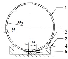
The structural scheme of theoretical model is created using real experimental model (Fig. 1). A hollow ball (No. 1) in theoretical model (Fig. 2) is considered as a full-standard, despite that a hollow ball in experimental model is cut. Its outside radius is 30 mm, wall thickness 1.5 mm and it is made of steel. According to that, the full ball moment of inertia $I$ (Eq. (1)) is equal to 73·10^-6 kg·m². The inside radius of piezo tube (No. 3) is 19.5 mm. The surface of the ball after a contact with a smart fluid (No. 4) becomes greasy. A sliding friction coefficient goes down, if the greasy surface comes over the zone of 3 contact points (No. 2). These points are made of epoxy resin that are located at 120° angle distance about tube longitudinal axis. Seeking to prevent from the coefficient reduction, the angular displacement of the ball must be constrained and the radius $R$ of the contact zone with a smart fluid has to be small enough. The horizontal projection of concave electrode (No. 5) is circle, which radius is 7.5 mm:

where $R_1$ – the outside radius of the ball; $t_1$ –the wall thickness of the ball; $\rho$ – the density of steel, which is 7850 kg/m³; $R$ – the radius of electrode horizontal projection; $t$ – the layer thickness of smart fluid, which is 0.5 mm.

The concave surface of the electrode is considered as flat, which contact area $A$ (Eq. (2)) is 1.77·10^-4 m². These initial angular speeds of the ball ${\omega }_0$ are: 0.2; 0.6 and 1 rad/s. According to this, the initial shear rates of smart fluid ${\gamma }_0$ (Eq. (3)) are: 12, 36 and 60 s^-1.

Fig. 1Experimental model

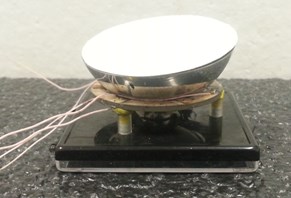
Fig. 2The structural scheme of theoretical model

3. Determination of ERF theoretical characteristics

To model the braking process electrorheological fluid LID 3354 s is chosen, which experimental and functional graphs are shown in Figs. 3 and 4 [5, 6]. Despite that a linear function is recommended to use for the dependence of ERF yield stress ${\tau }_Y$ versus electric field strength [5], but a quadratic function (Eq. (4)) is chosen in order to get similar forms of the graphs. A sample function of second degree (Eq. (5)) is used to approximate experimental dependence of ERF viscosity $\mu$ versus electric field strength [5]. ERF viscosity value is considered to be permanent, when speed gradient changes:

where $E$ – electric field strength; ${\mu }_0$ – initial ERF viscosity, when $E$ is equal to 0; $C_{\mu }$ – the constant of ERF viscosity function; $T$ – the response time of smart fluid.

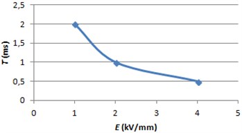
The average speed of ERF polarized particles is going up, until anizotropic structural block is created, when electric field strength is rising. This means, that the response time $T$ changes in accordance to $E$, when the layer thickness of the fluid is constant [5]. A parabolic function (Eq. (6)) is chosen to model the mentioned dependence (Fig. 5). Despite that, the nominal value of exterior electric field strength can be reached almost instantly, but in theoretical model is considered that the field strength is changing linearly till nominal value is reached over response time period.

GER fluid, which performance is explained by giant electrorheological effect, can be used in order to get higher values of yield stress [7].

Fig. 3ERF yield stress graphs

Fig. 4ERF viscosity graphs

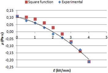
Fig. 5ERF response time graph

4. Determination of MRF theoretical characteristics

To model the braking process magnetorheological fluid 140CG is chosen. After the investigation of theoretical shear models [8] and MRF viscosity characteristic (Fig. 6) [9], Bingham model is selected. MRF shear because of viscosity ${\tau }_{\mu }$ (Eq. 7) doesn’t depend on the strength of magnetic field and almost linearly depends on shear rate. This means, that MRF viscosity value can be assumed as a constant.

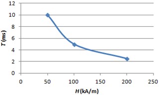
MRF yield stress ${\tau }_Y$ is depended on the strength of magnetic field, which experimental graph (Fig. 7) is approximated with quadratic function (Eq. (8)). Using the newest references about MRF [10] the dependence of response time versus magnetic field strength is created using parabolic function (Eq. (9)):

where $H$ – magnetic field strength.

Fig. 6MRF shear graphs because of viscosity

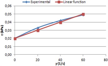
Fig. 7MRF yield stress graphs

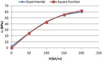
Fig. 8MRF response time graph

5. Functional model of the stepped approximation

The equivalent shear stress τ of smart fluid is evaluated using an Eq. (10). The initial kinetic energy $E_{K,pr}$ of the ball is determined using an Eq. (11). The dependence of the friction coefficient $f$ versus a sliding speed is evaluated in Eq. (12). The negative work because of friction $A_F$ is determined in Eq. (13) and negative work because of fluid shear $A_R$ – in Eq. (14). The final value of ball kinetic energy $E_K$ can be found using an Eq. (15). The model of the braking process is consisted of many time periods, when variable physical properties are recounted. The evaluation of the braking process is finished when the final value of the kinetic energy is equal to 0 Eq. (16). The total negative work after one time period shouldn’t be bigger than 10 % of the initial kinetic energy in order to get quite accurate results of the stepped approximation. The estimation of important kinematic properties is presented in Eqs. (17-20):

where $f_0$ – a sliding friction coefficient, when the sliding speed is infinitesimal, which value is 0.3 [11]; $N$ – the normal force in the friction zone, which is considered as permanent and equal to 1 N; $\mathrm{\Delta }t$ – a time period; $\mathrm{\Delta }s\left(t\right)$ – a braking distance at the time period $t-∆t\to t$; $s\left(t\right)$ – a total braking distance till a time moment $t$; $v\left(t\right)$ – a braking velocity at the time period $t\to t+∆t$; $a\left(t\right)$ – a braking acceleration at the time period $t-∆t\to t$.

6. Results

The essential properties of braking results using the chosen smart fluids are presented in Tables 1 and 2.

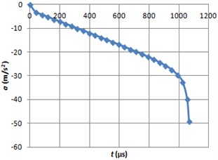
The graphs of the ball sliding distance, velocity and acceleration are shown (Fig. 9-14) when electrorheological fluid LID 3354 s (${\omega }_0=$ 0.6 rad/s and $E=$ 2 kV/mm) and magnetorheological fluid 140CG (${\omega }_0=$ 0.6 rad/s and $H=$ 100 kA/m) are used.

Fig. 9Braking path graph using ERF

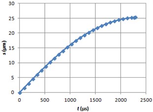
Fig. 10Braking velocity graph using ERF

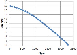
Fig. 11Braking acceleration graph using ERF

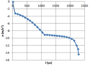
Fig. 12Braking path graph using MRF

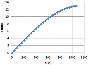
Fig. 13Braking velocity graph using MRF

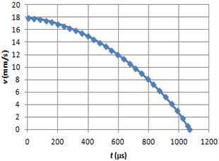
Fig. 14Braking acceleration graph using MRF

7. Conclusions

The braking times are very similar to the response times of LID 3354 s, when an initial angular speed of the ball is the lowest, according to the table 1 data. When the speeds of the ball are greater, then the braking times are several times longer than the appropriate response times. The braking times and distances differs approximately from 3 (${\omega }_0=$ 0.2 rad/s) to 5 (${\omega }_0=$ 1 rad/s) times when the strength value of electric field varies from the lowest to the highest.

The braking times using MRF don’t reach the appropriate response times, according to the Table 2. The braking times and distances differs approximately from 5 (${\omega }_0=$ 0.2 rad/s) to 10 (${\omega }_0=$ 1 rad/s) times when the strength value of magnetic field varies from the lowest to the highest.