Causes and classification of EMD mode mixing

1. Introduction

Since its introduction, Hilbert-Huang Transform [1] (HHT) has been widely used in many fields. The signal processing method is based on the hypothesis that a signal consists of a finite number of Intrinsic Mode Functions (IMFs). Up to now, researchers have not found any rigorous mathematical formula for decomposing signals into a finite number of IMFs. Instead, they have relied on a specific algorithm called Empirical Mode Decomposition (EMD). Although EMD is regarded by HHT researchers as a reliable method of obtaining the IMFs of a signal, it is plagued by some problems that require urgent solution [2-4]. One of the problems being intensively studied is the mode mixing that occurs during the process of EMD decomposition. Mode mixing refers to the situation when an IMF resulting from EMD decomposition has components of different frequencies. A lot of effort has been made on solving the mode mixing problem. Such as Huang, Senroy, Deering and so on [5-9]. They proposed their own solutions about the mode mixing based on their academic background. But they failed in identifying the real causes of mode mixing. As a result, the application scopes of the solutions proposed in these papers cannot be determined, which hinders wider application of these solutions.

Therefore, it is necessary to analyze and discuss the causes of mode mixing. Considering that EMD relies on the signal extrema to decompose signals, we start the investigation from the influence of the signal extrema on the EMD decomposition result, as well as from the relationship between the signal amplitude, the frequency variation, and the number of extrema. Then, we apply the findings in this study to analyze three widely-used solutions to the mode mixing problem and explore their strengths and drawbacks. The results of this study contribute to further EMD research.

2. Research on EMD mode mixing

A signal was constructed for investigating the relationship between its extrema and the EMD decomposition result. Two harmonic signals, $x_1$ and $x_2$ ($x_1$ is the high frequency signal). The impact of the signal extrema on the EMD decomposition result was studied by varying the amplitude and frequency of $x_2$. Two parameters are defined here, one is the ratio $K$ of the number of extrema of the low frequency signal to that of the composite signal $x$, and the other is the index which measures the result of decomposing the composite signal, which is defined as [10]:

where $x=x_1+x_2$, $c_1$ is the first order IMF obtained by decomposing $x$ using EMD decomposition. Obviously, $c_1$ corresponds to the high frequency signal $x_1$. It should be exactly or roughly as the same as $x_1$ when the decomposition produces a good result, and therefore $index\approx$ 0. If mode mixing occurs during the process of decomposition, then c1 will contain some components of $x_2$ or it will be roughly the same as $x$. Therefore, 0 $\le index\le$ 1. Without a loss of generality, signal $x_1$, $f_1=$ 1.5 Hz, $A_1=$ 1. The lengths of signals were in the range of 0-20 seconds and the step was 0.001 seconds.

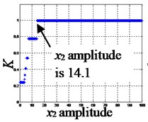
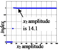
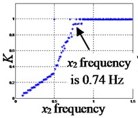
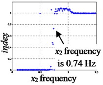
In the first Experiment 1, $A_2$ acted as the variable, and was in the range 0.1-100, step was 0.1, $f_2=$ 0.4 Hz. The experimental results are shown in Fig. 1(a), (b). As shown in Fig. 1(a), the ratio $K$ gradually increased accordingly. When $A_2=$ 14.1, $x$ became impossible to decompose, see Fig. 1(b). In the second Experiment 2, $f_2$ acted as the variable, and was in the range 0.09-1.49 Hz, step 0.01 Hz, $A_2=$ 3. The experimental results are shown in Fig. 1(c), (d). As shown in Fig. 1(c), the ratio $K$ increased gradually from 0.74 to approximately 1 (Fig. 1(c)). $x$ was almost impossible to decompose, see Fig. 1(d).

It can be seen from the variation of the two parameters of $K$ and index that when the number of extrema of the composite signal was equal to that of the low frequency signal, the EMD decomposition could not be accomplished. In Experiment 1, the time scale of the high frequency signal was overwhelmed due to the excessively large amplitude of the low frequency signal, which created a situation where the number of extrema of the composite signal was consistent with that of the low frequency signal. In Experiment 2, the waveform of the composite signal experienced the beat frequency phenomenon when the two frequencies became close to each other, which created a situation where the number of extrema of the composite signal was almost equal to that of the low frequency signal. In other words, the condition of the number of extrema of the composite signal being inconsistent with that of the low frequency signal was the reason why the signal could not be decomposed normally using the EMD.

Fig. 1K and index change with x2 parameters

a)

b)

c)

d)

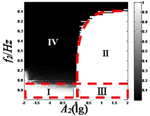
Harmonic signals have explicit mathematical expression and conform to the definition of IMF, whereas non-stationary signals are complex, and their expressions are diverse. Therefore, we used harmonic signals to illustrate the characteristics of different types of mode mixing. In the previous section, two experiments be used for analyzing the causes of mode mixing, they are far from sufficient for the classification of mode mixing. Here, the effectiveness of EMD decomposition was illustrated by a decomposition plane, and the classification of mode mixing were studied by observing the effects of amplitude and frequency variations of the low frequency signal. Refer to the references [10-13] for a description of the decomposition plane. Without a loss of generality, signal $x_1$, $f_1=$ 1 Hz, $A_1=$ 1, signal $x_2$, 0 $<f_2<$ 1, 0 $<A_2\le$ 10. Composite signals of different constituent frequencies and amplitudes could be constructed by varying $f_2$, $A_2$. The signal decomposition outcome diagram, index value, could be plotted according to the decomposition outcome corresponding to each pair of ($A_2$, $f_2$), see Fig. 2, $f_2$ is the $Y$-axis, $A_2$ is the $X$-axis (using their common logarithm values). According to the index value, the diagram can be roughly divided into 4 zones: Zone I: $A_2<$ 1, $f_2>$ 0.8 Hz the composite signal was almost impossible to decompose, Zone II:$A_2>$ 1, $f_2<$ 0.8 Hz the signal could not be decomposed too , it can be seen from the trend of the curve that the area of impossible to decompose always exists as the amplitude increases, Zone III: $A_2>$ 1, $f_2>$ 0.8 Hz, the signal could not be decomposed; Zone IV: $A_2<$ 1, $f_2<$ 0.8 Hz , the signal could be decomposed.

Zone I in Fig. 2 indicates that when the frequencies of the two signals were close enough (the ratio of low frequency to high frequency was greater than 0.8), the composite signal could not be decomposed, and this situation is not related to the magnitude of the signal amplitude. Zone II indicates that when the amplitude of the low frequency signal was greater than that of the high frequency signal, only a certain portion of the zone satisfied the conditions for successful signal decomposition, and the frequency of the signal could hardly make any difference under this condition. As both the phenomena of the frequencies getting too close and the amplitude of the low frequency signal being too large were present in Zone III, these two situations make the signal impossible to decompose. The experimental result in Fig. 2 shows that improper values of amplitude and frequency of the signal could cause mode mixing in EMD decomposition. Based on the above analysis and the current status of the EMD technique, this paper proposes to divide various forms of mode mixing into two basic types according to the causes, one type is caused by the frequencies of the signals getting too close, and the other type is caused by the excessively large amplitude of the low frequency signal. Different types of mode mixing require different solutions. Up to now, the distinction between different types of mode mixing and its consequences have not received much attention in the literature.

Fig. 2Decomposition plane showing outcome of EMD decomposition

3. Analysis of typical mode mixing solutions

By making use of the findings discussed earlier in this paper. This chapter explore the mechanisms of three mode mixing solutions.

3.1. Derivation method

The derivation method was first seen in [5]. Their paper mentions that some of the signals that cannot be decomposed by standard EMD method become decomposable after undergoing a derivation. However, the paper does not explain the mechanism of this method.

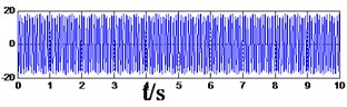
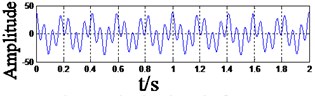
Suppose that the composite signal is composed of two harmonic signals: high frequency signal $x_1$, low frequency signal $x_2$, $f_1>f_2$, $A_1<A_2$. According to the repression of the harmonic signal, the amplitudes of the two harmonic signals become $A_1{\left(2\pi f_1\right)}^n$ and$A_2{\left(2\pi f_2\right)}^n$ after one or multiple derivations, $n$ is the number of derivatives. As $f_1>f_2$, there must be a larger-than-zero integer $m$ which makes $A_1{\left(2\pi f_1\right)}^m>A_2{\left(2\pi f_2\right)}^m$. In other words, after derivation, the amplitude of the high frequency signal becomes larger in relation to that of the low frequency signal, which means that the composite signal shifts from Zone II to IV on the diagram shown in Fig. 2. A series of experiments were conducted to verify the effectiveness of the derivation method in eliminating mode mixing. Let $f_1=$ 15 Hz, $A_1=$ 0.5, $f_2=$ 5 Hz, $A_2=$ 17, the duration be 2 s, the sampling interval be 0.001 s. The waveform of the original composite signal is shown in Fig. 3(a). After three rounds of derivation, the waveform becomes the one shown in Fig. 3(b). Next, the signal shown in Fig. 3(b) can be decomposed normally, indicating that the derivation method was effective in eliminating mode mixing.

However, there are two types of mode mixing, as described earlier in this paper. Aside from the type caused by amplitude imbalance, there is another type caused by the proximity of the frequencies of the constituent signals (corresponding to the Zones I and III in Fig. 2). The derivation method only changes the amplitude ratio between the two signals. It does not change the frequency ratio. So, the derivation method cannot deal with the mode mixing caused Zone III and Zone I. They were caused by frequency proximity.

Fig. 3The sum of difference harmonic wave and its third derivative

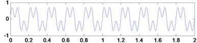
a) The synthetic signals of high and low frequency signals

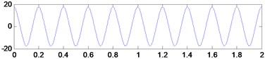
b) Three order derivation of synthetic signal

3.2. Frequency shifting method

With the aim of changing the ratio between the frequencies of two signals, the frequency shifting method refers to the use of complex number multiplication and division operations to achieve frequency addition and subtraction [6]. The application of this method requires a suitable reference frequency. The complex expression of each constituent signal of the composite signal is divided by the complex expression of the reference frequency to obtain a new frequency (this is equivalent to subtracting the frequency of the signal with the reference frequency). After frequency shifting, the frequency ratio between the two signals changes, and the order of the two signals is reversed in terms of frequency value. As can be seen from [6], when proposing the frequency shifting method, due to the lack of understanding in the classification of mode mixing, the author only explained how to deal with the type of mode mixing caused by frequency proximity and ignored the type of mode mixing caused by amplitude. According to the findings in this paper, this method is also applicable to the mode mixing caused by amplitude. Since the frequency ratio between the two signals changes and the order is reversed in terms of frequency value after frequency shifting (i.e., the original low frequency signal becomes the high frequency signal, and the mode mixing caused by amplitude is also prevented from occurring). The mechanism and application of this method are explained further below.

We assume the frequencies of the constituent signals are $f_1$ and $f_2$ respectively, $f_1$ > $f_2$. An appropriate reference signal is chosen whose frequency is $f$, and $f_1$ < $f$. The complex expression of each constituent signal is divided by the complex expression of the reference signal to realize frequency subtraction. See Eq. (2):

2

$\left|f_1-f\right|<\left|f_2-f\right|\Rightarrow \mathrm{\Delta }{f}_1⋖\mathrm{\Delta }{f}_2.$

The mathematical processing obviously changes the relation between the two constituent signals. The frequency ratio between the two signal changes from $f_2$/$f_1$ to $\mathrm{\Delta }{f}_1$/$\mathrm{\Delta }{f}_2$, which means the frequency ratio between the originally neighboring IMFs has changed. As discussed previously, mode mixing occurs when the frequency ratio between the two constituent signals reaches the level $f_2$/$f_1$ > 0.8 (corresponding to the Zones I and III in Fig. 2). When the ratio $\mathrm{\Delta }{f}_1$/$\mathrm{\Delta }{f}_2$ falls into Zone IV, i.e., less than 0.8, the mode mixing caused by frequency proximity can be avoided. Another change happens to the order of the frequencies of the original IMFs. As shown from Eq. (2), the order of the constituent signals is reversed in term of frequency value after frequency shifting, but the amplitude ratio between the two signals remains the same, which can be translated to a shift from Zone II to IV in Fig. 2.

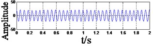
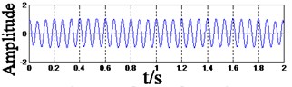
How to deal with the mode mixing caused by frequency proximity has been covered in [3]. Here we discuss how to tackle the mode mixing caused by an excessively large amplitude of the low frequency signal. Assume signal, $f_1=$ 15 Hz, $A_1=$ 1, $f_2=$ 5 Hz, $A_2=$ 17. The signal duration was 10 s, step 0.001 s. The reference frequency $f=$ 18 Hz, $A=$ 1. Fig. 4(a) shows the waveform of the composite signal before frequency shifting. In the waveform after frequency shifting shown in Fig. 4(b), the high frequency was 13 Hz, low frequency was 3 Hz. EMD could be accomplished because the amplitude of the high frequency signal was larger than that of the low frequency signal.

Fig. 4The synthetic signal with the high amplitude value, and the waveform after frequency shift

a) The synthetic composed of harmonic signals of 5 Hz and 15 Hz

b) The waveform after frequency shift by 18 Hz

3.3. Masking signal method

In this paper, if an IMF obtained through EMD decomposition was flawed by mode mixing, it is called pseudo IMF. When the harmonic composite signals in Zones I, II, and III in Fig. 2 were being decomposed by EMD, the resulting IMFs were typical pseudo IMFs. The detailed process of constructing the masking signal described in [7]. It shows that the average frequency calculated using the energy-weighted mean of IMF1 of the original signal was close to the frequency of IMF1, and the amplitude of the masking signal was large enough (1.6 times the original signal). As discussed in Chapter 2, a phenomenon like beat frequency can occur when the frequencies of the two signals are close to each other. The masking signal method can be explained by this paper discussed, A masking signal whose frequency is approximate to that of the to-be-separated constituent signal is constructed to produce beat frequency with the intermittent signal and obtain a pseudo IMF. The masking signal is eliminated later. If the amplitude of the masking signal is too small, it may interact with the low-order IMF to produce new pseudo IMFs, making it impossible to screen the crosstalk of the low-order IMF components during the breaks of signal. Therefore, the amplitude of the masking signal should be large enough to screen the low-order IMF components.

As discussed before, there are two types of mode mixing, one occurs when the frequencies of the constituent signals are too close to each other, and the other occurs when the amplitude of the low frequency signal is too large. Due to the lack of understanding in the causes and classification of mode mixing, [7] did not discuss the effectiveness of the masking signal method in dealing with the mode mixing caused by an excessively large amplitude of the low frequency signal. In fact, this method is applicable to this type of mode mixing. It is worth noting that enough space must be maintained between the instantaneous frequency corresponding to the pseudo IMF created by the masking signal method and the instantaneous frequency of the low-order IMF (i.e., the low frequency to high frequency ratio must not be greater than the frequency ratio in Zone I in Fig. 2). Only when this condition is satisfied can the low-order IMF component be completely screened. Fig. 5 shows an example of applying the masking signal method to handle mode mixing caused by excessively large amplitude of low frequency signal. Fig. 6(a) shows the waveform of a composite signal synthesized with two signals ($f_1=$ 15 Hz, $A_1=$ 1, $f_2=$ 5 Hz, $A_2=$ 17). The composite signal cannot be decomposed normally by EMD decomposition, because the amplitude of the low frequency signal is much larger than that of the high frequency signal. A masking signal whose frequency and amplitude are 17 Hz and 20 respectively is added to the composite signal to solve the mode mixing, and the composite signal is decomposed by EMD to obtain a pseudo IMF, see Fig. 5(b). After that, the masking signal is removed from the composite signal. The waveform of the resulting composite signal is shown in Fig. 5(c).

Fig. 6Using the masking signal method to eliminate mode mixing

a) The synthetic signal after adding masking signal

b) The pseudo IMF obtained by EMD decomposition signal

c) The waveform of pseudo IMF after removing masking signal

4. Conclusions

This paper analyzes the causes of mode mixing using the impact of the signal extrema on the result of EMD decomposition as a handle and identifies two basic types of mode mixing. Based on our findings about the causes of mode mixing, three typical mode mixing solutions were analyzed. Since the inventors of these solutions did not provide satisfactory explanations on the mechanisms of the solutions in their papers, this paper provides a detailed elucidation on how these solutions work on the two types of mode mixing and determines the application scopes of these solutions. Our findings regarding the causes and classification of mode mixing have been validated through experiments and may contribute to finding better solutions to mode mixing in EMD decomposition.