Circular-linear model of the force of dry friction

Ragulskis, K.; Bubulis, A.; Maskeliūnas, R.; Paškevičius, P.; Ragulskis, L.

doi:10.21595/mme.2018.20503

Mathematical Models in Engineering

Browse Journal

Submit article

Published: 31 December 2018

Check for updates

Circular-linear model of the force of dry friction

K. Ragulskis¹

A. Bubulis²

R. Maskeliūnas³

P. Paškevičius⁴

L. Ragulskis⁵

¹Kaunas University of Technology, K. Donelaičio Str. 73, LT-44249, Kaunas, Lithuania

²Kaunas University of Technology, Mechatronics Institute, Studentų Str. 56, LT-51424, Kaunas, Lithuania

³Vilnius Gediminas Technical University, Saulėtekio Al. 11, LT-10223, Vilnius, Lithuania

⁴Company “Vaivora”, Palemono Str. 2a, LT-52191, Kaunas, Lithuania

⁵Vytautas Magnus University, Vileikos Str. 8, LT-44404, Kaunas, Lithuania

Corresponding Author:

K. Ragulskis

Cite the article Download PDF

Downloads 1295

Abstract

In the numerical methods taking into account the force of dry friction numerical approximation is used when performing calculations. Circular-linear approximation for the local transition region is recommended. Results of numerical calculations are presented. The advantages of using this proposed representation are seen from the obtained results presented in this paper.

1. Introduction

When numerical methods are applied for nonlinear problems various types of procedures are used for approximation of nonlinear behavior of the system. In engineering applications it is important to take into account the force of dry friction. Various approximate representations of this phenomenon may be used. In this paper circular-linear approximation for the local transition region is proposed and investigated numerically.

This paper continues the investigations presented in [1] and [2]. Basic problems taking into account the force of dry friction and their analysis are presented in [3].

Problems of surface cleaning are described in [4]. This dynamical process is also presented in [5]. Particles and their interactions with surfaces are analyzed in [6]. Particles interacting with larger particles are investigated in [7]. Adhesion of particles is presented in [8]. Experimental investigations of particles are described in [9]. The force of dry friction is essential in the numerical analysis of models of cleaning of surfaces.

2. Circular-linear approximation of dry friction

Further $u$ denotes displacement of the investigated vibrating system, $H$ represents the approximate force representing dry friction and dot over the variable denotes differentiation with respect to the time $t$ .

Value of velocity at the beginning of the local transition interval between the constant values of the force is ${\dot{u}}_{1}$ and value of velocity at the end of the local transition interval between the constant values of the force is ${\dot{u}}_{2} .$ The average value is:

1

{\dot{u}}_{c} = \frac{{\dot{u}}_{1} + {\dot{u}}_{2}}{2} .

Value of the force approximating dry friction at the beginning of the local transition interval is $H_{1}$ and value of the force approximating dry friction at the end of the local transition interval is $H_{2} .$ The average value is:

2

H_{c} = \frac{H_{1} + H_{2}}{2} .

Further $r$ denotes small radius of the circle.

Case 1. It is assumed that:

3

H_{1} > H_{2} .

The following lengths are calculated:

4

s = \sqrt{{({\dot{u}}_{c} - {\dot{u}}_{1})}^{2} + {((H_{1} - r) - H_{c})}^{2}},

5

t = \sqrt{s^{2} - r^{2}} .

The following angles are calculated:

6

α = a r c t a n \frac{r}{t},

7

β = a r c t a n \frac{(H_{1} - r) - H_{c}}{{\dot{u}}_{c} - {\dot{u}}_{1}} .

The following coordinates of points are calculated:

8

{\dot{u}}_{3} = {\dot{u}}_{c} - t c o s (α + β),

9

H_{3} = H_{c} + t s i n (α + β),

10

{\dot{u}}_{4} = {\dot{u}}_{c} + t c o s (α + β),

11

H_{4} = H_{c} - t s i n (α + β) .

The circular-linear special function is defined as:

12

C ({\dot{u}}_{1}, {\dot{u}}_{2}, H_{1}, H_{2}, \dot{u}) = \{\begin{array}{l} H_{1} - r + \sqrt{r^{2} - {(\dot{u} - {\dot{u}}_{1})}^{2}}, & \dot{u} < {\dot{u}}_{3}, \\ H_{2} + r - \sqrt{r^{2} - {(\dot{u} - {\dot{u}}_{2})}^{2}}, & \dot{u} > {\dot{u}}_{4}, \\ H_{3} + \frac{H_{4} - H_{3}}{{\dot{u}}_{4} - {\dot{u}}_{3}} (\dot{u} - {\dot{u}}_{3}), & {\dot{u}}_{3} \leq \dot{u} \leq {\dot{u}}_{4} . \end{array}

Case 2. It is assumed that:

13

H_{1} < H_{2} .

The following lengths are calculated:

14

s = \sqrt{{({\dot{u}}_{c} - {\dot{u}}_{1})}^{2} + {(H_{c} - (H_{1} + r))}^{2}},

15

t = \sqrt{s^{2} - r^{2}} .

The following angles are calculated:

16

α = a r c t a n \frac{r}{t},

17

β = a r c t a n \frac{H_{c} - (H_{1} + r)}{{\dot{u}}_{c} - {\dot{u}}_{1}} .

The following coordinates of points are calculated:

18

{\dot{u}}_{3} = {\dot{u}}_{c} - t c o s (α + β),

19

H_{3} = H_{c} - t s i n (α + β),

20

{\dot{u}}_{4} = {\dot{u}}_{c} + t c o s (α + β),

21

H_{4} = H_{c} + t s i n (α + β) .

The circular-linear special function is defined as:

22

C ({\dot{u}}_{1}, {\dot{u}}_{2}, H_{1}, H_{2}, \dot{u}) = \{\begin{array}{l} H_{1} + r - \sqrt{r^{2} - {(\dot{u} - {\dot{u}}_{1})}^{2}}, & \dot{u} < {\dot{u}}_{3}, \\ H_{2} - r + \sqrt{r^{2} - {(\dot{u} - {\dot{u}}_{2})}^{2}}, & \dot{u} > {\dot{u}}_{4}, \\ H_{3} + \frac{H_{4} - H_{3}}{{\dot{u}}_{4} - {\dot{u}}_{3}} (\dot{u} - {\dot{u}}_{3}), & {\dot{u}}_{3} \leq \dot{u} \leq {\dot{u}}_{4} . \end{array}

The force of dry friction is approximated in the following way:

23

H = \{\begin{array}{l} C (- Δ, Δ, - h, h, \dot{u}), & |\dot{u}| < Δ, \\ h, & |\dot{u}| \geq Δ, \dot{u} > 0, \\ - h, & |\dot{u}| \geq Δ, \dot{u} < 0, \end{array}

where $h$ is the coefficient of dry friction, $Δ$ determines the width of the interval of transition between the values of the force of dry friction.

The following system is investigated:

24

m \ddot{u} + c \dot{u} + k u = P s i n ω t - H,

where $m$ is the mass, $c$ is the coefficient of viscous friction, $k$ is the stiffness, $P$ is the amplitude of the exciting force, $ω$ is the frequency of the exciting force.

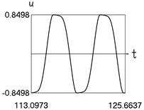
In the performed investigation values of the parameters of the system are: $ω =$ 1, $h =$ 3.2, $P =$ 4, $m =$ 1, $c =$ 0.1, $k =$ 1, $r =$ 0.15 $.$ Zero initial conditions were assumed. Steady state motion was investigated, and two periods were represented.

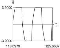
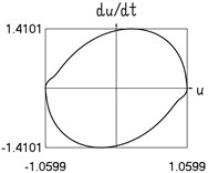
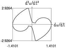
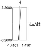
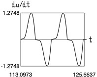
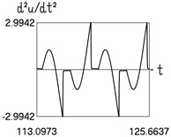
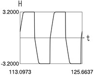
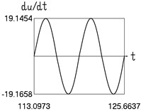
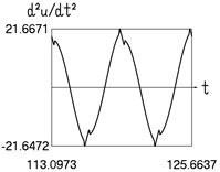
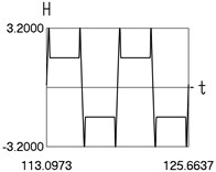
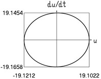
Results for $Δ =$ 0.8 are shown in Fig. 1.

Fig. 1Dynamics in steady state regime (wide transition region)

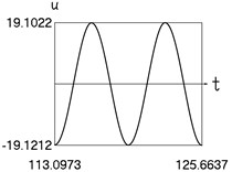
a) Displacement and time

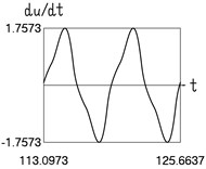
b) Velocity and time

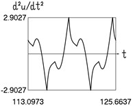
c) Acceleration and time

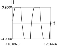
d) $H$ and time

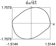
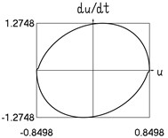
e) Velocity and displacement

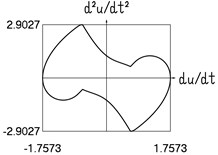
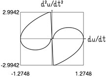
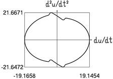
f) Acceleration and velocity

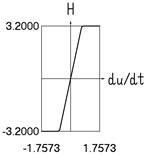
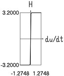
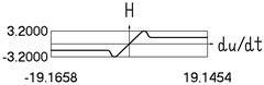
g) $H$ and velocity

Results for $Δ =$ 0.4 are shown in Fig. 2.

Fig. 2Dynamics in steady state regime (transition region of medium width)

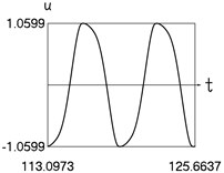
a) Displacement and time

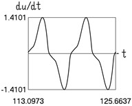
b) Velocity and time

c) Acceleration and time

d) $H$ and time

e) Velocity and displacement

f) Acceleration and velocity

g) $H$ and velocity

Results for $Δ =$ 0.2 are shown in Fig. 3.

Fig. 3Dynamics in steady state regime (narrow transition region)

a) Displacement and time

b) Velocity and time

c) Acceleration and time

d) $H$ and time

e) Velocity and displacement

f) Acceleration and velocity

g) $H$ and velocity

Three typical widths of the transition region are investigated. Typical results are presented. The effect of the width of the transition is seen from the obtained numerical results.

3. More complicated model of dry friction

The coefficient of dry friction increases in the vicinity of the value of zero velocity. It is assumed that $\frac{h}{Δ} = \frac{h_{a}}{Δ_{a}}$ , where $h_{a}$ denotes the increase in the coefficient of dry friction, $Δ_{a}$ defines the width of the transition interval connecting the values of the coefficient of dry friction $h$ and $h + h_{a} .$ It follows that $h_{a} = h \frac{Δ_{a}}{Δ} .$

The force of dry friction is approximated in the following way:

25

H = \{\begin{array}{l} C (- Δ - Δ_{a}, Δ + Δ_{a}, - h - h \frac{Δ_{a}}{Δ}, h + h \frac{Δ_{a}}{Δ}, \dot{u}), & |\dot{u}| < Δ + Δ_{a}, \\ C (Δ + Δ_{a}, Δ + 2 Δ_{a}, h + h \frac{Δ_{a}}{Δ}, h, \dot{u}), & Δ + Δ_{a} \leq |\dot{u}| < Δ + 2 Δ_{a}, \dot{u} > 0, \\ C (- Δ - 2 Δ_{a}, - Δ - Δ_{a}, - h, - h - h \frac{Δ_{a}}{Δ}, \dot{u}), & Δ + Δ_{a} \leq |\dot{u}| < Δ + 2 Δ_{a}, \dot{u} < 0, \\ h, & |\dot{u}| \geq Δ + 2 Δ_{a}, \dot{u} > 0, \\ - h, & |\dot{u}| \geq Δ + 2 Δ_{a}, \dot{u} < 0 . \end{array}

In the performed investigation values of the parameters of the system are: $ω =$ 1, $h =$ 1.6, $Δ =$ 1.8, $Δ_{a} =$ 1.8, $P =$ 4, $m =$ 1, $c =$ 0.1, $k =$ 1, $r =$ 0.8. Zero initial conditions were assumed. Steady state motion was investigated and two periods were represented.

Results are shown in Fig. 4.

Dynamics of the system with more complicated model of dry friction is seen from the obtained numerical results.

Fig. 4Dynamics in steady state regime (more complicated model of dry friction)

a) Displacement and time

b) Velocity and time

c) Acceleration and time

d) $H$ and time

e) Velocity and displacement

f) Acceleration and velocity

g) $H$ and velocity

4. Conclusions

When performing numerical analysis of engineering problems in which the force of dry friction is essential for the representation of behavior of the dynamical system some type of numerical approximation is used in the process of calculations. In this paper circular-linear approximation for the local transition region is investigated. The advantages of using this proposed representation are seen from the presented graphical results.

Three typical widths of the transition region are investigated. Typical results are presented. The effect of the width of the transition is seen from the obtained numerical results.

In the more complicated model of dry friction the coefficient of dry friction increases in the vicinity of the value of zero velocity. Dynamics of the system with more complicated model of dry friction is seen from the graphically presented numerical results.

On the basis of the obtained numerical results circular-linear approximation of dry friction is recommended for calculations in the investigations of engineering problems. Among those problems the investigations of processes of surface cleaning are essential.

References

Ragulskis K., Bubulis A., Paškevičius P., Pauliukas A., Ragulskis L. Investigation of elliptical approximation in the model of the force of dry friction. Mathematical Models in Engineering, Vol. 4, Issue 3, 2018, p. 151-156.

Publisher
Ragulskis K., Paškevičius P., Bubulis A., Pauliukas A., Ragulskis L. Improved numerical approximation of dry friction phenomena. Mathematical Models in Engineering, Vol. 3, Issue 2, 2017, p. 106-111.

Publisher
Sumbatov A. S., Yunin Ye. K. Selected Problems of Mechanics of Systems with Dry Friction. Physmathlit, Moscow, 2013, (in Russian).

Search CrossRef
Chahine G. L., Kapahi A., Choi J.-K., Hsiao Ch.-T. Modeling of surface cleaning by cavitation bubble dynamics and collapse. Ultrasonics Sonochemistry, Vol. 29, 2016, p. 528-549.

Publisher
Witte A. K., Bobal M., David R., Blättler B., Schoder D., Rossmanith P. Investigation of the potential of dry ice blasting for cleaning and disinfection in the food production environment. LWT – Food Science and Technology, Vol. 75, 2016, p. 735-741.

Publisher
Petean P. G. C., Aguiar M. L. Determination of the adhesion force between particles and rough surfaces. Powder Technology, Vol. 274, 2015, p. 67-76.

Publisher
Cui Y., Sommerfield M. Forces on micron-sized particles randomly distributed on the surface of larger particles and possibility of detachment. International Journal of Multiphase Flow, Vol. 72, 2015, p. 39-52.

Publisher
Jiang Y., Turner K. T. Measurement of the strength and range of adhesion using atomic force microscopy. Extreme Mechanics Letters, Vol. 9, Issue 1, 2016, p. 119-126.

Publisher
Kumar N., Zhao C., Klaassen A., Van Den Ende D., Mugele F., Siretanu I. Characterisation of the surface charge distribution on kaolinite particles using high resolution atomic force microscopy. Geochimica et Cosmochimica Acta, Vol. 175, 2016, p. 100-112.

Publisher

About this article

Received

30 October 2018

Accepted

13 December 2018

Published

31 December 2018

DOI

https://doi.org/10.21595/mme.2018.20503

Keywords

circular-linear approximation

force of dry friction

numerical results

vibrations

graphical representation

Acknowledgements

The authors thank the reviewers for providing ideas and valuable comments. They enabled to improve the presentation in the paper.

This is an open access article distributed under the Creative Commons Attribution License, which permits unrestricted use, distribution, and reproduction in any medium, provided the original work is properly cited.

Previous article in issue Previous Next article in issue Next

Research article

2022 02 05

Kinematic and dynamic analysis of three-mass oscillatory system of vibro-impact plate compactor with crank excitation mechanism

Vitaliy Korendiy, Oleksandr Kachur, Volodymyr Gursky, Volodymyr Gurey, Nadiia Maherus, Oleh Kotsiumbas, Oleksandr Havrylchenko

Research article

2019 09 30

Radiation damping for rigid foundations. Approximate expressions

Bertha Olmos, José Manuel Jara, Guillermo Martínez

Research article

2019 04 25

Comparison of the performance of friction pendulums with uniform and variable radii

Cristian-Tatian Malin, Dorian Nedelcu, Gilbert-Rainer Gillich, Adrian Petrica, Ioan Padurean

Research article

2018 09 30

Investigation of elliptical approximation in the model of the force of dry friction

K. Ragulskis, A. Bubulis, P. Paškevičius, A. Pauliukas, L. Ragulskis

K. Ragulskis, A. Bubulis, R. Maskeliūnas, P. Paškevičius, and L. Ragulskis, “Circular-linear model of the force of dry friction,” Mathematical Models in Engineering, Vol. 4, No. 4, pp. 210–215, Dec. 2018, https://doi.org/10.21595/mme.2018.20503

Copy Extrica

Copied to clipboard!

TY  - JOUR
DO  - 10.21595/mme.2018.20503
UR  - https://doi.org/10.21595/mme.2018.20503
TI  - Circular-linear model of the force of dry friction
T2  - Mathematical Models in Engineering
AU  - Ragulskis, K.
AU  - Bubulis, A.
AU  - Maskeliūnas, R.
AU  - Paškevičius, P.
AU  - Ragulskis, L.
PY  - 2018
DA  - 2018/12/31
PB  - JVE International Ltd.
SP  - 210-215
IS  - 4
VL  - 4
SN  - 2351-5279
SN  - 2424-4627
ER  - 

Copy Ris

Copied to clipboard!

@article{Ragulskis_2018,
	doi = {10.21595/mme.2018.20503},
	url = {https://doi.org/10.21595/mme.2018.20503},
	year = 2018,
	month = {dec},
	publisher = {{JVE} International Ltd.},
	volume = {4},
	number = {4},
	pages = {210--215},
	author = {K. Ragulskis and A. Bubulis and R. Maskeli{\={u}}nas and P. Pa{\v{s}}kevi{\v{c}}ius and L. Ragulskis},
	title = {Circular-linear model of the force of dry friction},
	journal = {Mathematical Models in Engineering}
}

Copy Bibtex

Copied to clipboard!

[1]K. Ragulskis, A. Bubulis, R. Maskeliūnas, P. Paškevičius, and L. Ragulskis, “Circular-linear model of the force of dry friction,” Mathematical Models in Engineering, vol. 4, no. 4, pp. 210–215, Dec. 2018, doi: 10.21595/mme.2018.20503.

Copy IEEE

Copied to clipboard!

Ragulskis, K., A. Bubulis, R. Maskeliūnas, P. Paškevičius, and L. Ragulskis. “Circular-Linear Model of the Force of Dry Friction.” Mathematical Models in Engineering 4, no. 4 (December 31, 2018): 210–15. https://doi.org/10.21595/mme.2018.20503.

Copy Chicago

Copied to clipboard!

Circular-linear model of the force of dry friction

Abstract

1. Introduction

2. Circular-linear approximation of dry friction

3. More complicated model of dry friction

4. Conclusions

References

About this article

Related Articles