Use of viscous fluid dampers for the improvement of the seismic response of RC structures

1. Introduction

The leading concept of seismic design procedures is based on guaranteeing the safety and functionality of the structures, avoiding collapse; this requires that certain elements take a dissipate energy through inelastic cyclic deformations. In this case, the damage might be required to occur and depending on its magnitude, structures may not be repairable, or the structural retrofitting may entail an important time. Structures of strategic importance for society (hospitals, fire stations, etc.) are critical since they require full-service continuity after an earthquake. Sometimes, the most conventional approach to protect structures against the effects of earthquakes is to increase both strength and stiffness. This approach is not always effective, as the stiffness increase may result in the amplification of seismic forces.

In order to study the advantages coming from the use of VFD, this paper is focused on the possible recurses to such as strategy in the structural design of an RC hospital building in Colombia. The structural design of the analyzed building, located in an intermediate seismic hazard zone, was performed according to the Colombian seismic design code. The requirement which is typical of hospitals, of operation continuity after a seismic event involves a challenge for structural engineers to implement special resources allowing optimal designs. In this case, an effective solution is given by the use of passive devices such as VFD, in order to have better control on the seismic response and reduce the demand for energy dissipation in structural elements.

The main focus of the study was to show the advantage of using nonlinear VFD, which allow a reduction in the damage level of the building over seismic loads. To do so, it was necessary to study the initial behavior of the building to determine the damage level without dampers. Finally, it was possible to define the location of the devices which lead the structure to a lower ductility demand.

2. Viscous fluid damper (VFD) as seismic protection devices

As already mention VFD is a passive control device. In this category, the devices are intended to operate without external power sources and have properties that cannot be modified during the seismic response of the structure. Since seismic input energy is contained in a relatively narrow frequency band, passive systems have been shown to be effective, robust and economical solutions.

The VFD devices dissipate energy through the relative velocities that occur between their connected points. The force-displacement response of these dampers usually depends on the frequency of the motion. Also, the forces generated by these devices in the structure are usually out-of-phase with the internal forces resulting from shaking. Therefore, the maximum forces generated by the dampers do not occur simultaneously with the maximum internal forces corresponding to the peak transient deformations of the structure [1]. A brief description for this device is a high resistance cylinder containing a fluid belonging to the silicone family and a piston with small holes on the edges of one of its heads. Then, under a seismic event, a piston slide is generated inside the cylinder, causing the transfer of fluid from one chamber to another, thus generate the damping force. Finally, the internal displacement of the piston allows the conversion of kinetic energy into heat producing thermal expansion and contraction of the fluid.

3. Case study

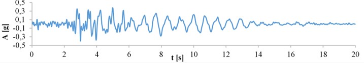
A 15th-story and one heliport RC building modelled as 3D is analyzed with and without VFD using ETABS software. The appropriate way to define these devices is by making use of “link elements” selecting the “Damper – Exponential” option. As it is known, a damper works on the axis direction of the device and the nonlinear viscous damper devices are being used. After computing the values of the damper, it is possible to add the required input parameters: stiffness, damping, and damping exponential. VFDs were located only in a diagonal configuration.

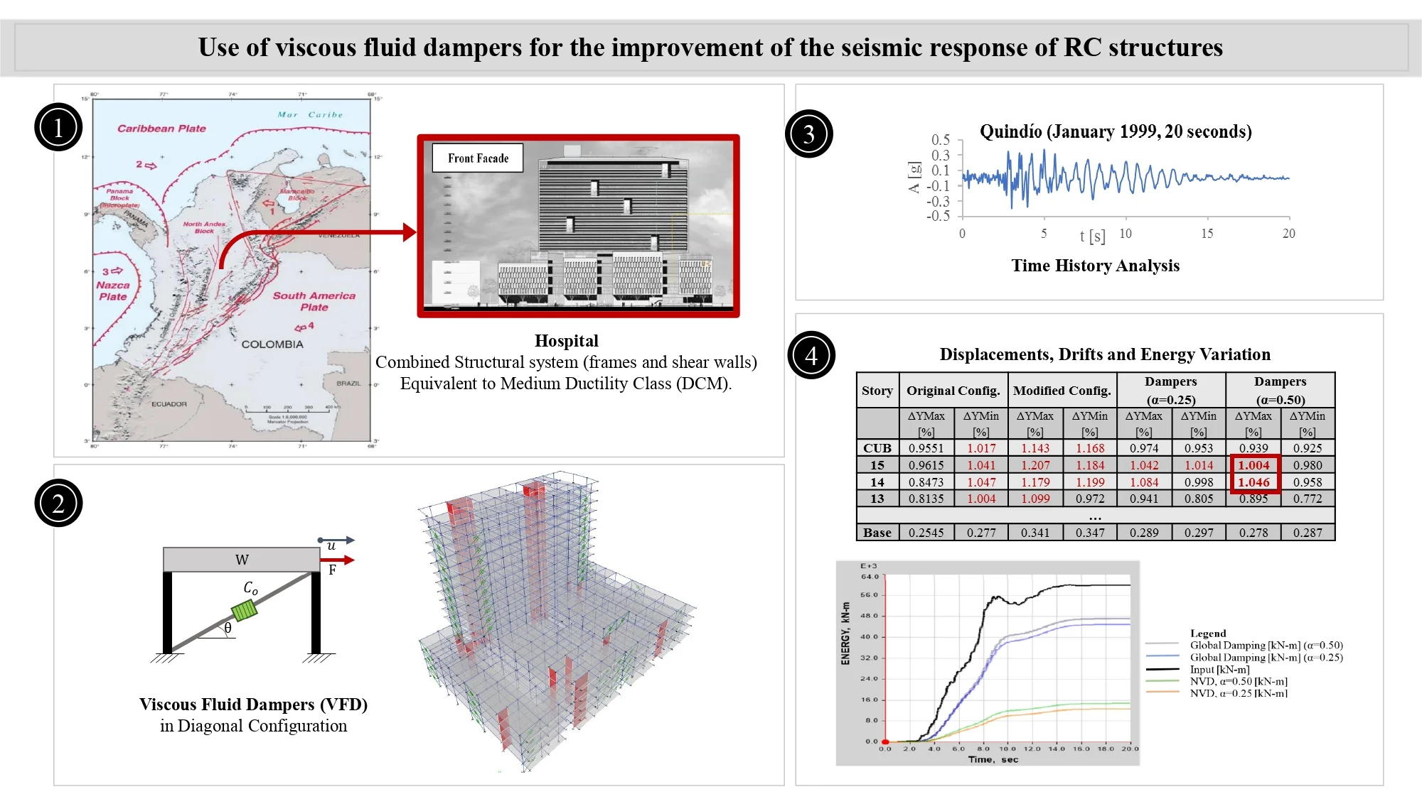
The dynamic load applied over the structure was simulated by a nonlinear time-history analysis (FNA) of the Quindío earthquake (Colombia, January 1999). The time-history data of the ground motion is presented in Fig. 1, which was a significant one for Colombia, affecting directly the country; PGA was scaled to 0.4 g, an acceleration value which ensures the activation of the dampers.

The implementation of the nonlinear analysis of the time-history is mandatory for this type of passive devices because seismic vibrations induce deformation beyond the yield limit in one or more structural elements.

Additionally, for the design, construction, and installation of the nonlinear VFD, the Maximum Considered Earthquake (MCE) shall be used [3]. Following this, Colombian seismic code requires that the MCE is 1.5 times the Design Basis Earthquake (DBE); therefore, for the design of the damping devices, the ground motion record was scaled to 0.6 g.

Fig. 1Quindío ground motion record (January 1999, 20 seconds)

3.1. Dampers location

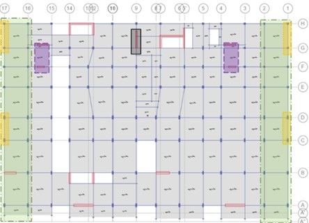
The best location of the viscous dampers is achieved through an iterative process, in which the designer must try different arrangements and locations considering the architecture and the use of the building. In this document, it was followed the ASCE 7-10 [4] recommendations for placing the dampers, which includes: the use of at least two devices in the direction to be reinforced, the placement of dampers in all the story levels, and the seek for symmetry to avoid torsion (see Fig. 2(a). It is worth mentioning that although dampers were placed in both directions ($X$ and $Y$), later on, in Chapter 4, it is explained the reason why in this document only the results and discussion will be presented based on the most critical direction, $Y$. Fig. 2(b) shows the distribution in $Z$-$Y$ direction that was considered for the final analysis.

Fig. 2a) 3D Model with VFDs, b) Z-Y view, without walls

a)

b)

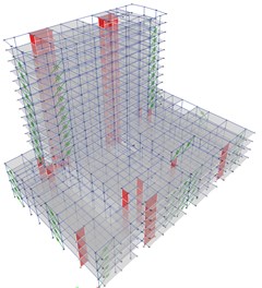
Before placing dampers in the structure, this was modified in order to get maximum advantage from the use of them. Due to the high number of walls, which provide too much rigidity to the building, it was decided to remove some of them in order to enhance the role played by dampers, ensuring maximum effectiveness. In general, the proposed modification implies the lengthening of four horizontal walls (axes 16-15 and 4-3) for the first stories (2nd-5th) and removed for the following levels (6th-roof), this with the purpose of giving continuity to the columns at their edges without altering the beam distribution in the upper floors. In addition, a fifth wall located at axis 9 was removed from the whole structure.

Because viscous dampers are velocity dependent devices, the distribution criterion throughout the building was based upon the points which show the highest velocities. Finally, considering the geometry configuration and all the criterion for the location of dampers, in the $Y$ direction, the same number of dampers were placed on the gridlines which are at the largest an equal distance either side from the center of mass, thus, at the building borders. Fig. 3 shows, for stories 2 and 6, the modifications done in the wall arrangement, together with the zones where the maximum velocities are presented and the final location of the dampers, accurately selected in order to resist torsion as well. Therefore, the structure will respond to a nonlinear relationship between force and deformation.

Fig. 3Final distribution of the dampers for a) story 2 and b) story 6

a)

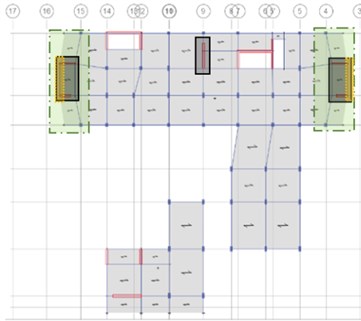
b)

4. Viscous damping devices design properties

In order to compute the viscous damping coefficient $C$ of each device, it was necessary to define the value for the whole structure; this was done by inverting Eq. (2). Firstly, the principal modes of the modified structure (with a change in geometry and some walls removed) were identified in order to define the modal parameters required for the computation of the $C_{tot}$. Table 1 provides period and effective modal mass values for the first 3 modes.

It can be observed that the first mode is in the $Y$ direction, the second one is a rotational mode, and the third mode is in the $X$ direction. For this case study, the analysis and results were focused on the direction of the most significant mode. Additionally, the added damping ratio selected for the direction of study, ${\xi }_{dY}$, was 25 %, and the amplitude $A_Y$, computed with the MCE signal record, was 432.78 mm.

The selection of an appropriate $\alpha$ is based on experience and typically design firms conduct trial-and-error design iterations [5]. Therefore, with the purpose of a better comparison, the procedure was done for a damping exponent of 0.25 and 0.50. Hence, by setting $\alpha$ exponent to 0.25, the lambda parameter takes a value of 3.70, and the total viscous damping coefficient, ∑$C_{d1}$, is 29176.67 kN-(s/m)^α; while for $\alpha$ of 0.50, $\lambda$ is 3.50, thus providing ∑$C_{d1}$, of 58846.73 kN-(s/m)^α.

In order to spread the total damping coefficient over the structure, a standard methodology based on the proportional distribution of the shear force (VD), was employed.

5. Results

5.1. Displacements and drifts

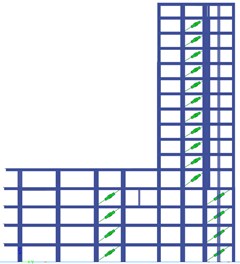
For the adopted seismic signal, floor displacements were obtained for each of the two earthquake cases (MCE and DBE). In addition, both the original and modified configuration were considered, with two different types of VFD, characterize by $\alpha$ of 0.25 and 0.50, respectively. It should be remembered that the VFD devices are used for the modified structure. Finally, for the DBE a good behavior was guaranteed by the activation of the dampers. Thus, higher results are expected in the MCE case.

It is possible to observe graphically in Fig. 4 that the VFDs are working in the correct way and in general terms, it is possible to see a reduction in the displacements.

Fig. 4Displacement direction Y – Quindío DBE

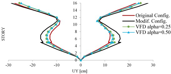
Table 2Drifts comparison direction Y – Quindío DBE

Story	Original configuration		Modified configuration		Dampers ($\mathrm{\alpha }=\mathrm{}$0.25)		Dampers ($\mathrm{\alpha }=\mathrm{}$0.50)
	$\mathrm{\Delta }{Y}_{Max}$ [%]	$\mathrm{\Delta }{Y}_{Min}$ [%]	$\mathrm{\Delta }{Y}_{Max}$ [%]	$\mathrm{\Delta }{Y}_{Min}$ [%]	$\mathrm{\Delta }{Y}_{Max}$ [%]	$\mathrm{\Delta }{Y}_{Min}$ [%]	$\mathrm{\Delta }{Y}_{Max}$ [%]	$\mathrm{\Delta }{Y}_{Min}$ [%]
CUB	0.9551	1.017	1.143	1.168	0.974	0.953	0.939	0.925
15	0.9615	1.041	1.207	1.184	1.042	1.014	1.004	0.980
14	0.8473	1.047	1.179	1.199	1.084	0.998	1.046	0.958
13	0.8135	1.004	1.099	0.972	0.941	0.805	0.895	0.772
12	0.1054	0.483	0.354	0.153	0.313	0.208	0.31	0.207
11	0.2443	0.083	0.61	0.443	0.462	0.312	0.436	0.285
…
3	0.586	0.617	0.793	0.793	0.669	0.674	0.641	0.652
2	0.5276	0.562	0.71	0.715	0.601	0.607	0.577	0.587
Base	0.2545	0.277	0.341	0.347	0.289	0.297	0.278	0.287

After performing the analysis in the Y direction, it was possible to appreciate that better results are obtained with a larger $\alpha$ value. Drifts were computed for each signal in the DBE case. Note that the maximum drift value allowed by the design code is 1 %. Table 2 presents the drift values, taking into account the original and modified structure, and the two $\alpha$ cases of VFD.

In general terms, it was not possible to fulfill the maximum drift required by the design code in all the top stories, where the drift was greater than 1 %. However, the maximum percentage is 1.084 %, which is very close to the limit value allowed in the design code.

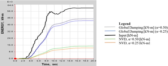
5.2. Structural system energy

The energy balance plot is particularly useful in order to see how energy is transferred to the supplemental damping systems. For the two different $\alpha$, the energy variation is shown in Fig. 5.

Since the purpose of adding supplemental damping is to dissipate energy, it is natural to consider the migration of energy quantities. The difference when using different $\alpha$ can be observed. For $\alpha =$0.50, the amount of energy dissipated by the devices is higher than the one obtained for $\alpha =$0.25.

Fig. 5Energy variation in direction Y – Quindío DBE

6. Conclusions

As expected, the use of the VFD reduces the structural displacements causing them to come close to the original configuration; additionally, it is possible to determine that, even when few values of drifts do not meet the 1 % requirement, with a higher $\alpha$, 0.50, in this case, lower displacements and therefore reduced interstory drifts are obtained

A reduction in the ductility level can be observed with the use of dampers. This can be evidenced in the energy variation graph, in which by increasing the $\alpha$, more energy is dissipated by the structure.

In this research work, the design approach for the proper use of damping devices consists basically in the traditional trial-and-error iterative process. Analyzing the effects of the distribution methodology which was used, it can be seen that satisfactory results can be achieved, in the sense that all devices are activated.

References

-
Soong T. T., Spencer Jr B. F. Supplemental energy dissipation: state-of-the-art and state-of-the-practice. Journal of Engineering Structures, Vol. 24, 2002, p. 243-259.
FEMA 274, Commentary to NEHRP Guidelines for the Seismic Rehabilitation of Buildings. Building Seismic Safety Council, Federal Emergency Management Agency, Washington, DC. 1997.
AIS 180-13, Recommendations for Seismic Requirements of Different Building Structures. Colombian Seismic Engineering Association, Bogotá, Colombia, 2013.
ASCE 7-10, Minimum Design Loads for Buildings and Other Structures. American Society of Civil Engineers, Reston, VA., 2010.
FEMA P-1052, 2015 NEHRP Recommended Seismic Provisions: Design Examples. Building Seismic Safety Council, Federal Emergency Management Agency, Washington, DC., 2016.
About this article