A technique for estimating geometrical synchronization of biomedical signals

1. Introduction

Evaluation of synchronization between data signals is a broadly discussed concept among researchers since it can be applied in the analysis of a wide range of phenomena. Several examples include analysis of biomedical signals in health sciences and biological systems, investigation of coupled circuits or laser systems in electronics and optics [1-3].

In [4, 5] we proposed a technique capable of estimating the degree of geometrical synchronization via near-optimal chaotic attractor embedding. In this paper, the measure is demonstrated and validated using the example of two coupled chaotic logistic maps. The technique is then applied to assess the impact of Earth’s local magnetic field on individual’s biomedical parameters.

2. Estimation of geometrical synchronization between two time series

Geometrical similarity between two time series can be estimated via the algorithms developed and validated in [4, 5]. A brief overview of those algorithms is presented below. The feasibility of the discussed approach is demonstrated by considering two logistic maps with diffusive coupling:

where $a=b=\text{4}$ (such parameter values result in chaotic behavior); $0\le \epsilon \le \text{1}$ is the coupling parameter (low values of $\epsilon$ result in low synchronization between maps and vice versa). Initial conditions are set to $x_0=\text{0.3}$ and $y_0=\text{0.6}$.

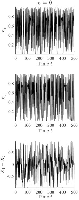
Two resulting trajectories $x=\left(x_1,\dots ,x_N\right)$, $y=\left(y_1,\dots ,y_N\right)$ of size $N=$ 6000 are sampled using Eq. (1) after transient processes die down. Fig. 1(a) illustrates the evolution of $x$ and $y$and the difference $x-y$ when two logistic maps are uncoupled ($\epsilon =0$). Fig. 1(b) depicts $x$, $y$, and $x-y$ when $\epsilon =\text{0.13}$ and Fig. 1(c) corresponds to $\epsilon =\text{0.16}$. It can be seen that the similarity between trajectories $x$ and $y$ increases as the coupling parameter $\epsilon$ increases; however, the difference $x-y$ remains chaotic even at $\epsilon =\text{0.16}$ (see Fig. 1).

Fig. 1The trajectories of coupled logistic maps (see Eq. (1)) for different values of the coupling parameter ε. Parts a), b) and c) illustrate x,y and x-y at ε=0, ε=0.13 and ε=0.16 respectively

a)

b)

c)

In order to evaluate geometrical synchronization between $x$ and $y$, both data signals are split into $m=\text{20}$ equal-sized segments of size $n=\text{300}$. The resulting segments $x_i^{\left(s\right)}$, $y_i^{\left(s\right)}$, $i=1,\dots ,m$ are then mapped onto integers ${\tau }_i^{*x}$, ${\tau }_i^{*y}$, $i=1,\dots ,m$ denoted as optimal time lags using the steps below:

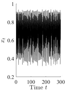
1) Let $z=(z_1,\dots ,z_n)$ be a data signal of size $n$ (corresponding to one of the segments) (see Fig. 2(a)).

2) Embed data signal $z$ into a 2D delay coordinate space using parameter $\tau \in \{1,\dots ,n-1\}$ as follows:

The obtained set of the embedded points is called an attractor (see Fig. 2(b)).

3) Compute the area of reconstructed attractor using the following formula for each $\tau =1,\dots ,200$:

4) Determine the optimal time lag ${\tau }^{*}$ resulting in the largest area of the attractor (see Fig. 2(c)):

It was shown in [4, 5] that the optimal time lag ${\tau }^{*}$ can be used as a scalar feature representing the geometrical properties of the analyzed data signal.

Fig. 2Part a) depicts one segment of data signal x displayed in Fig. 1(b). Parts b) and c) illustrate the corresponding reconstructed attractors at τ=4 and τ*=63 (optimal time lag), respectively

a)

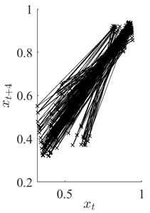
b)

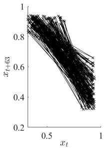
c)

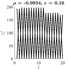
Geometrical synchronization between data signals $x$ and $y$ is then estimated as the Pearson correlation coefficient between optimal time lag vectors ${\tau }_{}^{*x}$ and ${\tau }_{}^{*y}$. Optimal time lags for $x$ and $y$ are represented in Fig. 3 for three values of coupling parameter $\epsilon$. It can be seen that the correlation between sequences of optimal time lags is $\rho =$ 0.1759, $\rho =$ 0.5714 and $\rho =$ –0.9934 at $\epsilon =$ 0, $\epsilon =$ 0.13 and $\epsilon =$ 0.16 respectively. Obtained results show that described geometrical synchronization estimation algorithm based on the optimal attractor embedding is able to detect the similarity between two chaotic data signals in an effective and efficient way.

Fig. 3Optimal time lag vectors τ *x (solid line) and τ *y (dashed line) corresponding to ε=0, ε=0.13 and ε=0.16 (parts a), b), c) respectively)

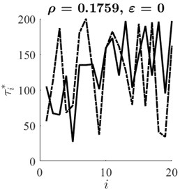
a)

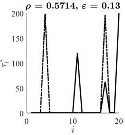
b)

c)

3. Estimation of synchronization between human heart rate variability and Earth’s local magnetic field

3.2. Application of the synchronization estimation algorithm

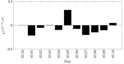
The geometrical synchronization measure presented in the previous section was applied to the experiment data to estimate the degree of synchronization between RR interval time series and the spectral power of local magnetic field. Note, that parameter $n$, denoting the length of data segments for the attractor embedding was selected to correspond to 5 minutes of data since it is the standard time span for the analysis of human heart rate variability (HRV). Fig. 4 displays mean synchronization values between all participants’ HRV and magnetic field power computed for each day of the experiment. Obtained synchronization values can be further analyzed with regards to magnetic field activity at a given date in order to investigate the impact of the geomagnetic field on human heart activity.

Fig. 4Mean synchronization between RR data series and magnetic field power for each day of the experiment

4. Conclusions

A technique for the estimation of geometrical synchronization between two data series using optimal attractor embedding is validated in this paper via the example of two coupled chaotic logistic maps. Presented technique is then applied to the real data in order to evaluate the degree of synchronization between human HRV and Earth’s geomagnetic activity.

References

-
Dörfler F., Bullo F. Synchronization in complex networks of phase oscillators: a survey. Automatica, Vol. 50, Issue 6, 2014, p. 1539-1564.
Quiroga R. Q., Kraskov A., Kreuz T., Grassberger P. Performance of different synchronization measures in real data: a case study on electroencephalographic signals. Physical Review E, Vol. 65, Issue 4, 2002, p. 041903.
González-Miranda J. M. Amplitude envelope synchronization in coupled chaotic oscillators. Physical Review E, Vol. 65, Issue 3, 2002, p. 036232.
Timofejeva I., McCraty R., Atkinson M., Joffe R., Vainoras A., Alabdulgader A., Ragulskis M. Identification of a group’s physiological synchronization with earth’s magnetic field. International Journal of Environmental Research and Public Health, Vol. 14, Issue 9, 2017, p. 998.
Timofejeva I., Poskuviene K., Cao M., Ragulskis M. Synchronization measure based on a geometric approach to attractor embedding using finite observation windows. Complexity, Vol. 2018, 2018, p. 8259496.
About this article