Analysis of traveling wave based fault location method for distribution network with image processing

1. Introduction

Distribution networks widely distribute anywhere we live. It has closest relationship to our production and daily life. However, earth faults almost occur every day for a municipal scale medium voltage distribution network. Actually, before applying an advanced fault location technology into practice, the physical inspection line is still a commonly used way to locate fault even though it requires additional manpower and costs a large amount of time. For fault location technologies, the traveling wave-based method has wide application for transmission networks. This method is based on traveling wave propagating at high speed and capturing the wave front at terminals of the transmission line. However, the traveling wave-based method faces tough challenge for distribution networks fault location due to much-branched structure and weak traveling wave signal so that it has been paid much attention to worldwide.

In [1] a model built and modified for a partial discharge propagation through underground medium voltage cables using Universal Line Model in order to improve the detection and location performance of the on-line partial discharge monitoring system. References [2-4] applied, evaluated and revised the electromagnetic time-reversal for fault or disturbances location. Reference [5] achieve accurate location of the fault section and fault distance with a multi measuring points method. References [6-8] studied and improved the traveling wave method. In [9] a fault location scheme based on network topology information and circuit breaker reclosure-generating travelling waves was proposed. However, this scheme is unable to perform the fault location function when the relate circuit breaker rejects act. Reference [10] proposed an on-line time reversal (OTR) approach which is able to locate faults in live transmission line networks. At the moment, weak traveling wave signal and expensive devices are the major difficulties the traveling wave methods faces for application.

This paper analyzed the principle of earth fault location with the traveling wave-based method for medium voltage distribution networks. Then given a specific tree structure of a distribution network, an image of nodes voltage is created and the dynamic changes of it are analyzed. On this basis, laws of traveling wave data from all nodes are discussed and summarized. The contribution of this paper lays the foundation for the future applied research on intelligence fault location algorithm.

2. Theory of traveling wave data analysis

A single-phase earth fault occurs at line section between $s_i$ and $s_j$ shown in Fig. 1. The traveling wave is then generated and propagates along the line.

Fig. 1Simple faulty line section

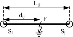
Traveling wave meters located at two ends of the line record the time $t_i$ and $t_j$ when the traveling wave are captured. The distance $d_{ij}$ from fault point to end of line $S_i$ can be then calculated by Eq. (1):

where $c$ is the propagation velocity of traveling wave.

A straight-line equation derived from Eq. (1) in slope-intercept form is then given by Eq. (2):

where $∆t$ is the difference between $t_i$ and $t_j$.

The position relationship between the fault point $F$ and the line section are classified into four categories.

1) When the fault point locates on or beyond the left end of the line section, $F\le 0$ is defined;

2) When the fault point locates between the two ends of the line section, $0<F<L$ is defined;

3) When the fault point locates on the right end of the line section, $F=0$ is defined;

4) When the fault point locates beyond the right end of the line section, $F>L$ is defined;

where $L$ is the total length of the line section.

Four straight line equations are plotted in a coordinate system where the horizontal axis represents $∆t_{ij}$, the difference time when first wavefront arrives at the ends $i$ and $j$ of the line section respectively, while the vertical axis represents $L_{ij}$, the length of line section between the nodes $i$ and $j$ shown in Fig. 2.

It is clearly known that the absolute value of the slope of the straight line equals the value of the propagation velocity of traveling wave from Fig. 2. When the fault point $F$ locates between the two ends of the line section, the value of the intercept of the corresponding straight line equals the distance $d_{ij}$ between node $i$ and fault point $F$.

The propagation velocity $c$ is then obtained by Eq. (3):

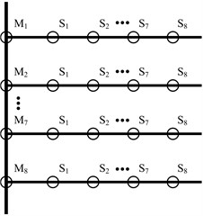
The Fig. 3 shows a distribution network with eight branches from number $M_1$ to number $M_8$. Nine traveling wave meters are deployed to each branch line and main line.

Fig. 2The straight line dependent on the location of fault point F

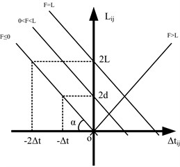
Fig. 3Distribution network with eight branches

According to Fig. 3 an array related to the distance $L_{ij}$ between any two different points on the same branch is designed shown in Fig. 4. Similarly, the Fig. 5 shows that the distance between any two points on the main line. The transmission node is one type of node connected to two lines and this node is a research object in Fig. 4. The fork node is another type of node connected to three lines and this node is a research object in Fig. 5. It is clearly known that $L_{ij}$ equals $L_{ji}$ and $L_{ij}$ equals 0 when node number $i$ equals $j$.

Fig. 4Array related to the distance between any two nodes on the same branch Mi (i ranges from 1 to 4)

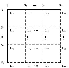
Fig. 5Array related to distance between any two nodes on the main line

The value of each element of these arrays represents that of voltage of the first wavefront. While the related coordinates represent the distance between corresponding nodes. Then the voltage distribution of the network can be represented with an image at some point. Aiming at some line the figures like Fig. 2 can also be plotted. The laws of these data can be then found and analyzed easily.

3. Simulation results

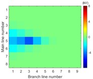
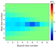
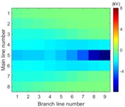
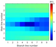
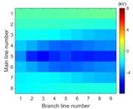
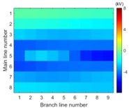
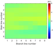
Simulation model for Fig. 3 is built. The single-phase solid earth fault occurs at the node number 5 of the main line. The total length of main line is 30 kilometers and the rated voltage is 10.5 kV. When each branch is arranged in each row of image data array and the amplitude of voltage of the first wave front represents the pixel of image, the simulation results in image form are then shown in Fig. 6.

The images from Fig. 6 clearly illustrate that the first traveling wave front is generated when the single-phase solid earth fault occurs and then propagates along the lines. Due to refraction and reflection of traveling wave, the amplitude of first wave front may be less than the later one so that the sensitivity of the fault location system is one of key factors to improve the reliability of fault location.

Fig. 6Simulation results in image form at the time

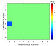
a) 5.00 ms

b) 5.01 ms

c) 5.02 ms

d) 5.03 ms

e) 5.04 ms

f) 5.05 ms

g) 5.06 ms

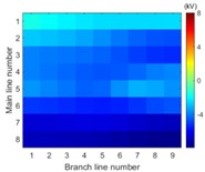
h) 5.10 ms

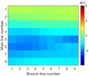
i) 5.20 ms

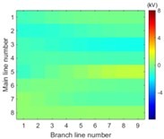
j) 5.30 ms

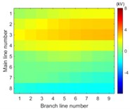
k) 5.35 ms

l) 5.40 ms

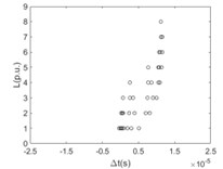
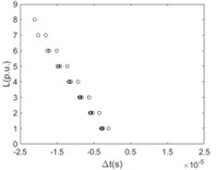
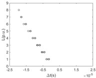
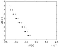
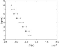
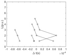
The time difference $∆t$ when the first traveling wavefront arriving at any two nodes of the same branch line with the relationship of the distance $L$ between these two nodes is shown in Fig. 7.

Fig. 7The difference between time ∆t with the relationship of the distance L (per unit based on actual length of the line section unit) at any two points of the same branch line numbered by 1-8 and respectively when sensitivity of the fault location system ksens is 0.1 times of rated voltage

a) 1

b) 2

c) 3

d) 4

e) 5

f) 6

g) 7

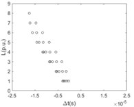
h) 8

It is clearly known from Fig. 7 that for the majority of branch lines the true data can be measured and distributed along straight line evenly. The absolute slope of this line equals the propagation velocity of the traveling wave. That the intercept of this straight line equals zero means that the point $F$ locates on or beyond the left end of this branch line. The nonlinear and random distribution of results in Fig. 7(a) indicates that when the sensitivity is given the branch near the side of voltage source is hard to locate fault by using travelling-wave based method due to limitation to the voltage magnitude of incipient wave front by the voltage source. This unexpected case can be also seen directly and clearly from the changes of pixels in the top row of each image in Fig. 6.

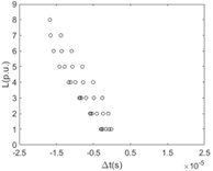
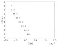
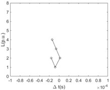
Similarly, the time difference $∆t$ when the first traveling wavefront arriving at any two nodes of the main line with the relationship of the distance $L$ between these two nodes is shown in Fig. 8. For the case that the sensitivity is equal to 0.1 times of rated voltage, a bunch of polylines are plotted regularly. As a matter of fact, the poly lines consist of two intersecting straight lines where the slope of one straight line is negative and the slope of another one is positive. For the negative slope of one of the intersecting straight lines, the intercept of this line is 2 times of the distance between the reference node and the fault point. With the value of the sensitivity increasing the polylines becomes sharpened and the turning points of them become obvious.

Fig. 8The difference between time ∆t with the relationship of the distance L (per unit based on actual length of the line section unit) at any two points of the main line when the sensitivity of the fault location system, ksens, equals 0.1, 0.2, 0.3, 0.4, 0.5, and 0.6 times of rated voltage respectively

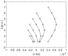
a) 0.1

b) 0.2

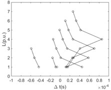
c) 0.3

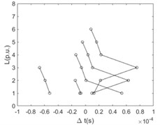
d) 0.4

e) 0.5

f) 0.6

4. Conclusions

1) Due to the traveling wave propagating along connected lines, the information of the first wave front can be measured from majority of nodes of the network in terms of proper sensitivity.

2) Propagation velocity and distance between reference nodes and fault point as two main parameters of fault location with traveling wave-based method can be extracted according to the laws of the data of the first wave front.

3) The reliability of the fault location can be improved as the available sensitivity increasing.