Abstract
The nonlinear aeroelastic vibrations of the Windbelt System are described in the paper. The system works based on aeroelastic flutter principle. The long narrow ribbon with pinned supports at the ends is used as mechanical model. The analysis of aerodynamic forces for a thin rectangular cross-section of the ribbon is provided. Lateral-torsional oscillations of the system is derived, considering aerodynamic forces. Conditions for generation of oscillations are determined using Poincaré-Andronov-Hopf bifurcation. The critical speed, which defines dynamic instability (aeroelastic flutter), is determined as well. The influence of the tension force and other ribbon parameters on the critical speed is considered. The supercritical behavior of the system is investigated.
Highlights
- The mathematical model for the lateral-torsional oscillations of a flexible ribbon under the influence of oncoming air flow is derived and analyzed.
- They describe the dynamics of a Wind belt type wind generator in a simplified form.
- Small lateral-torsional oscillations of the system are analyzed.
- The value of the critical velocity, the trajectory of motion, and the bifurcation diagram are obtained.
1. Introduction
Wind energy is one of the main areas of alternative energy. It is based on conversion of kinetic energy of the air masses into electrical, mechanical or thermal power. The transformation of airflow energy into electrical energy is usually accomplished through wind turbines. Recently, the possibility of producing electric energy using a wind generator, called “Wind Belt” [1-5], is being intensively studied.
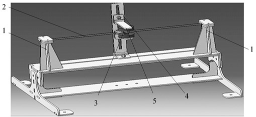
The schematic diagram of the device is shown in Fig. 1; taken from [3]. A permanent magnet 3 is fixed on a flexible tape 2 stretched between two rigid supports 1 (constructions with two or more magnets are also known [1]). Inductance coils 5 are arranged coaxially with the magnet on top and bottom of the ribbon on the frame 4. The airflow can disturb the static balance of the ribbon and lead to the excitation of its oscillation as an aeroelastic flutter [6] under certain conditions. The vibrating movement of the magnets induces current in nearby pickup coils, which subsequently can be rectified to a direct voltage.
Fig. 1Schematic diagram of a wind generator “Windbelt”
There are a few studies related to the generation of electric current in such devices in the existing scientific literature. However, investigation of the oscillations of a thin ribbon depending on its tension and the airspeed has been studied insufficiently. Known computational models are based on various simplified assumptions that limit investigation of supercritical behavior based on bifurcation analysis.
The purpose of this work is to model the dynamics of the ribbon in the air flow, analyze its movement and the possibility of structure optimization.
1.1. Problem statement
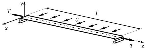
A ribbon of length with hinged supports on both ends is positioned in the oncoming air flow (Fig. 2). It is stretched by the longitudinal force along the axis. The cross section of the ribbon is constant along the length. The ribbon in horizontal air flow of constant rate has lifting force (wind load), which is evenly distributed along the length.
The net lifting force is applied along a line that passes through the pressure centers of cross section. This line is parallel to the -axis at a distance (Fig. 2).
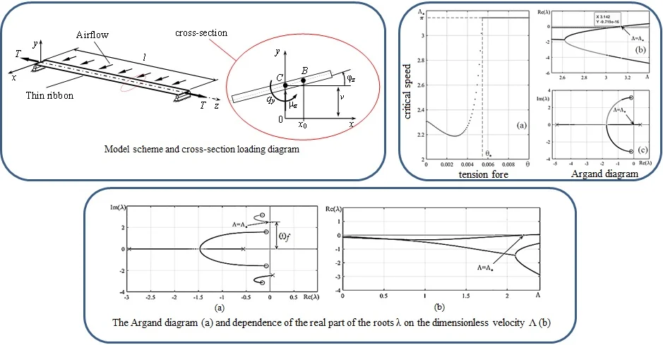
Fig. 2a) Model scheme and b) cross-section loading diagram
a)
b)
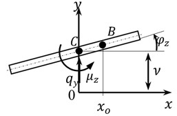
The lifting force is distributed over length and applied to the center of pressure line (point in Fig. 2) [6], where is the density of the environment, is the width of the cross section of the ribbon, – is lifting force coefficient. The lifting force point is relocated to the center of the cross section, point . To compensate this transition, the force system is supplemented by linear torques .
The lifting force coefficient for a thin rectangular profile of the ribbon is given by a known solution for a flow of an ideal incompressible fluid , where , are the expansion coefficients, is the effective angle of attack, is the vertical movement of the ribbon axis (pole).
1.2. Equations of motion
The motion of the considered model is described by a system of equations for lateral-torsional oscillations of a string on hinged supports, which is loaded with distributed force and distributed moment [7]. Taking into account the relocation of lifting forces to the center of gravity and the expression for the lifting coefficient, the system becomes:
where is the density of the ribbon, is the shear modulus, is area of cross section, is the polar moment of inertia, – is geometric stiffness of the section (strip) during torsion, , – is linear viscous Rayleigh damping coefficients in bending and torsion, respectively.
Further, Eq. (1) is reduced to a dimensionless form. Whereupon, dimensionless parameters are introduced: time , deflection , coordinate , velocity , force , and scales , , , , . The systems of Eq. (1) take the form:
All of them are expressed in terms of two fixed dimensionless parameters and :
Damping coefficients are equal to 5 % of its critical value ( is mode number).
1.3. The calculation of the critical speed
The system of Eq. (2) is reduced to a system with a finite number of degrees of freedom using the Galerkin method. The solution is represented in the form of an expansion on the basis where are functions satisfying the boundary conditions for the considered model (Fig. 2). The constant is determined from the condition of basis property and orthonormality of functions .
After applying the Ritz-Galerkin method Eq. (2) will take the form:
where .
The existing trivial solution of the Eq. (3) corresponds to the equilibrium position, which is defined as an unperturbed motion. The Eq. (3) is linearized near the equilibrium position for stability analysis. Then, the Eq. (3) in matrix form:
Solutions of the Eq. (4) are sought in the form . Then, the characteristic equation to determine takes the form . Further, the solution is considered only for the first mode (1) with the following parameter values 0.002, 0.03.
The dimensionless tension force is set in a way that the dynamic loss of stability occurs earlier than the static one (divergence). Otherwise, there is a divergence phenomenon when torsional rigidity of the ribbon is completely lost.
Fig. 3(a) shows the dependence of the critical velocity on the tension force . When a certain value of the tension force is reached, the critical speed becomes equal to and does not grow with further increase of . This value of the critical velocity corresponds to divergence. This is confirmed by Fig. 3(b) and Fig. 3(c) when (○ – beginning of trajectory, × – trajectory end). The first trajectory intersects the axis at in the value (Fig. 3(b)) that corresponds to the transition of the same trajectory through the origin at the Argand diagram (Fig. 3(c)). It corresponds to static loss of stability.
Fig. 3a) The dependence of the critical speed Λ* on the tension force θ; b) the dependence Reλon Λ; c) static stability loss on the Argand diagram
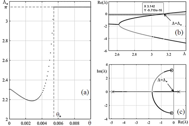
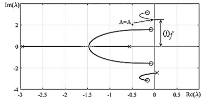
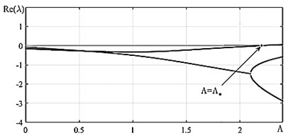
An analysis of the results shows that the parameter must be in the range of in order to observe dynamic loss of stability before static one. Here, it is defined as 0.002. Fig. 4(a) shows trajectories of roots for selected parameters. The point of their transition to the right half-plane is determined. The system has a critical velocity value at this point.
The value of the imaginary part has the meaning of the oscillation frequency of the system at . The value of corresponds to the ordinate of the marked point in Fig. 4(a). The value of is defined by dependence of the real part of the roots on (Fig. 4(b)), at the point equals zero 2.203.
Fig. 4a) The Argand diagram and b) dependence of the real part of the roots λ on the dimensionless velocity Λ; ○ – beginning of trajectory, × – trajectory end
a)
b)
1.4. Analysis of supercritical behavior
To study supercritical behavior the nonlinear system (see Eq. (3)) is integrated. A speed value greater than by 10 % is used. The motion is considered at the dimensionless time interval , where is the wave number for the frequency .
Numerical simulation of the Eq. (3) shows that periodic solutions can be established, i.e., there are both unstable equilibrium position and stable periodic motions in the supercritical region.
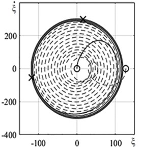
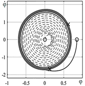
To evaluate the establishment of a self-oscillatory regime, phase portraits in Fig. 5(a) and Fig. 5(b) of vertical dimensionless movement and dimensionless rotation of the cross-section from the Eq. (3) are derived for different initial conditions: 1) , 2) .
The attractions of the trajectories to the limit cycles are clearly visible in Fig. 5.
Fig. 5Phase portraits for coordinate functions at a) ζ= 1/2 lateral oscillations ξ˙,ξ and b) torsional oscillations φ˙, φ; “ –– “ – trajectory with initial conditions No. 1; “– – –“ – trajectory with initial conditions No. 2; ○ – beginning of trajectory, × – trajectory end
a)
b)
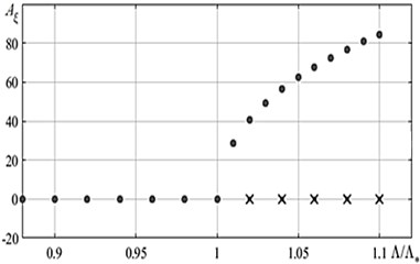
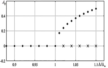
The analysis of stability of the equilibrium rectilinear position of the tape allows to plot a bifurcation diagram (Fig. 6). It was shown above that there are stable periodic motions in the supercritical, region that corresponds to a stable branch on the bifurcation diagram. Numerical integration by establishing method is utilized to plot the diagram, [8]. The results for the amplitudes and are presented in Fig. 6(a) and Fig. 6(b), respectively.
Fig. 7The bifurcation diagram a) for ξ and b) for φ: ● – stable motion, × – unstable motion
a)
b)
2. Conclusions
The mathematical model for the lateral-torsional oscillations of a flexible ribbon under the influence of oncoming air flow is derived and analyzed. The value of the critical velocity, the trajectory of motion, and the bifurcation diagram are obtained. Small lateral-torsional oscillations of the system are analyzed. They describe the dynamics of a Windbelt-type wind generator in a simplified form. The calculations show that there is a hyperbolic law.
References
-
Frayne S. Generator Utilizing Fluid Induced Oscillations. Patent US7573143 B2, 2009.
-
Windbelt Cheap Micro Wind Generator, http://www.reuk.co.uk/wordpress/wind/windbelt-cheap-micro-wind-generator/.
-
Vu Dinh Quy, Nguyen van Sy, Dinh Tan Hung, Vu Quoc Huy Wind tunnel and initial field tests of a micro generator powered by fluid-induced flutter. Energy for Sustainable Development, Vol. 33, 2016, p. 75-83.
-
Bibo A., Li G., Daqaq M. F. Electromechanical modeling and normal form analysis of an aeroelastic micro power generator. Journal of Intelligent Material Systems and Structure, Vol. 22, Issue 6, 2011, p. 577-592.
-
Bryant M., Garcia E. Modeling and testing of a novel aeroelastic flutter energy harvester. Journal of Vibration and Acoustics, Vol. 133, Issue 1, 2011, p. 011010.
-
Fung Y. C. An Introduction to the Theory of Aeroelasticity. Wiley, New York, 2008.
-
Vibrations in Tehnique, Vol. 1: Linear Systems Oscillations. Moscow, Mashinostroenie Publ, 1978, p. 352, (in Russian).
-
Nayfeh A. H., Mook D. T. Nonlinear Oscillations. Wiley, New York, 1979.
About this article

The work is supported by the Russian Science Foundation (project No. 18-19-00708).
