Vibration and aeroelastic control of wind turbine blade based on B-L aerodynamic model and LQR controller

1. Introduction

Flap bending-Lag bending-twist (BBT) flutter in dynamic stall state is an important reason of fatigue damage for wind turbine blades. How to effectively realize aeroelastic control has become an important research needed to be investigated in the last few years. For the active aeroelastic control methods of blades, one category is load reduction based on structural trailing edge flap, microtab and piezoelectric actuator [1-4], the other is the direct application of intelligent control theories [5]. Although in these works, the blade properties dynamically represent a real rotor blade; the analytical object is the flap-wise or torsional behavior of a helicopter blade or the vibration behavior of a wing airfoil in which stall nonlinear flutter of BBT coupling action is not mentioned.

Gebhardt et al. present an aeroelastic system of three-blade wind turbines which results from the coupling of aerodynamic model and a structural model based on a segregated formulation derived in an index-based notation [6]. However, the viscous effects of aerodynamic model in [6] can be confined to those regions close to solid surfaces, which is unable to study in depth the stall condition. Wang et al. present a nonlinear aeroelastic model for large wind turbine blades by combining blade element momentum theory and mixed-form formulation of geometrically exact beam theory [7]. However, compared with the solution of the aerodynamic analytical model (such as B-L model), the error of calculation result is still a little large. Khazar et al. present load mitigation of bending-twist coupling blade based on aeroelastic tailoring via unbalanced laminates [8]. Compared with the bending-twist coupling study of aeroelastic tailoring blade, research on BBT coupling is more general especially in some stall divergent cases. Dong et al. do predict BBT coupling blade loads based on the CFD and CSD solvers, but it is in a loosely coupled manner [9]. As for aeroelastic intelligent control, Boukhezzar et al. provide comparison between linear and nonlinear control strategies for variable speed wind turbines [10]. However, stall flutter is not involved in [10].

In present work vibration and aeroelastic control of stall nonlinear flutter of wind turbine blade with BBT coupling have been investigated for composite single-cell thin-walled structure based on B-L aerodynamic model [11-12] and linear quadratic controller (LQC). In view of the usual circumstances, there being a variable pitch motion in wind turbine, the structural equations are complicated and include nonlinear terms. The solution of stability analysis is also a complex process with nonlinear aeroelastic equations linearized. To simplify analysis, a set of BBT coupling models for composite rotating blade are considered, with constant pitch angle set. The analysis is applied to a laminated construction of symmetric layup beam structure with NACA 6315 aerofoil profile. The B-L stall aerodynamic model is applied based on the method of fitting static elastic coefficients to avoid the aerodynamic decomposition along blade span. The stall nonlinear flutter stability and LQC aeroelastic control effects based on different parameters are analyzed here by dynamic responses.

2. Equations of motions

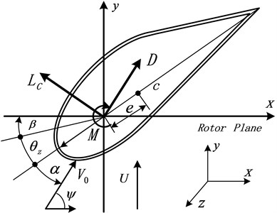
The single-cell thin-walled composite structure is widely used in construction of wind turbine blade for theoretical study. Fig. 1 shows the blade sectional parameters and aerodynamic forces. The sectional middle-line expression of the aerofoil profile is approximately described as [13]:

The origin of the rotating system ($x$, $y$, $z$) is located at the rigid root. The motions of blade beam have three degrees of freedom: flap bending direction, denoted by $y$, lag bending direction perpendicular to flap, denoted by $x$, and twist motion by ${\theta }_z$, with constant pitch angle of the whole blade $\beta$ set. The relative wind angle is denoted by $\psi$. The mass per unit length is $m$. The chord length is $c=$1 m. The thickness of blade section is denoted by $h$, and the distance 1/4 chord length by $e$. Tip speed ratio $\lambda =$6. The wind velocity is denoted by $U$. The length of the blade is $L=$15 m in $z$ direction and it has the constant rotating speed $\mathrm{\Omega }=\lambda U/L$, normal to the plane of rotation. Nonlinear aerodynamic lift is denoted by $L_C$, drag by $D$, and moment by $M$ respectively. The composite properties of blade are: the circumferentially symmetric layup configuration used here consists of ${\left[\theta \right]}_{2n}$ in both the top side above the chord, and the bottom side, with ply number being 10, ply thickness being 1.27×10^-3m; the maximum exterior height perpendicular to chord direction is 1.506×10^-1m, blade density $\rho =$1672 kg/m³, and $G_{12}=$3.5 GPa, $v_{12}=$0.34, $E_{11}=$ 25.8 GPa, $E_{22}=$8.7 GPa.

Fig. 1Blade section parameters and aerodynamic forces

Present analysis is formulated to estimate the characteristics of rotating blade with elastic coupling by means of a simplified deflection theory (SDT) [14]. The SDT method is developed for predicting the effective elastic stiffnesses and corresponding load deformation behavior of tailored composite box-beams. Based on SDT analysis for symmetric layup design and configuration, with constant pitch angle set, the BBT motions here with aerodynamic action are obtained respectively as follows:

Flap-wise motion:

Lag-wise motion:

Twist motion:

where the items of aerodynamic forces are in the right-hand-side; $K_x$, $K_{\theta }$, and attack angle $\alpha$ are defined respectively as:

Herein, $K_{22}$ is the chordwise shear stiffness; $K_{25}$ is the spanwise bending-chordwise shear coupling stiffness; $K_{46}$ is the chordwise bending-torsion coupling stiffness; $K_{55}$ is the spanwise (flap) bending stiffness; $K_{66}$ is the chordwise (lag) bending stiffness. The expressions of stiffness parameters $K_{ij}$ and the parameters of principle mass radii of gyration of blade cross section, $K_{m1}$, $K_{m2}$, $K_m$, are given as:

where the elements of the ply stiffness matrix ${\stackrel{-}{Q}}_{ij}$ are defined in texts discussing macro-mechanical behavior of composite piles [14].

3. B-L dynamic stall aerodynamic model based on fitting static elastic coefficients

The unsteady aerodynamic model, one example is the B-L model, is firstly used to describe the unsteady aerodynamic forces on an airfoil undergoing arbitrary motion in a flow [11, 12]. The occurrence of stall flutter of wind turbine blade leads to the need for analysis of unsteady aerodynamic forces in the stalled region. The B-L dynamic stall aerodynamic model of unsteady aerodynamics based on fitting static elastic coefficients is suggested here. The structural model in Eqs. (2-4) is coupled to the B-L model through the aerodynamic forces [11, 12]:

where the unsteady lift coefficient $C_L^{dyn}$, the unsteady drag efficient $C_D^{dyn}$, and the unsteady moment coefficient $C_M^{dyn}$ are approximately expressed as:

were, ${\alpha }_0$ is the angle of attack at zero lift, $C_{L,\alpha }$ is linear lift slope coefficient, $f^{st}$ is the separation point function, $C_L^{fs}$ is the lift coefficient of fully separated flow, $a^{st}$ is the arm to equivalent pressure centre. The variable $x_{a2}$ satisfies the following equation:

where ${\alpha }_f=x_{a1}/C_{L,\alpha }+{\alpha }_0$, and the variable $x_{a1}$ satisfies the equation:

and $C_L^p$ is the unsteady lift coefficient for attached flow.

Very few applications of B-L model are taken into account spanwise effects, with B-L model originally formulated in the state-space. During the conventional aerodynamic integration process of the aerodynamics given by the right-hand-side terms in Eq. (2-4) in the application of Galerkin method, aerodynamic decomposition is often carried out in place of the integral calculus with sum operation. Hence the tremendous computing workload can embarrass the real-time display in computer environment.

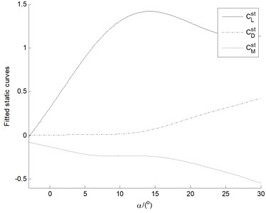
In order to simplify computation, we developed an approach of fitting static elastic coefficients based on experimental data of testing modeling of NACA 6315 aerofoil to reduce order of nonlinear equation, and linearize and simplify aeroelastic stability analysis [15]. The fitted static elastic coefficients $C_L^{st}$, $C_D^{st}$, and $C_M^{st}$, as the 8-degree polynomial of the attack angle $\alpha$, are expressed in polynomial formulas as:

where the related coefficients $p_i$($i=$ 1, 2,…, 9) are listed in Table 1.

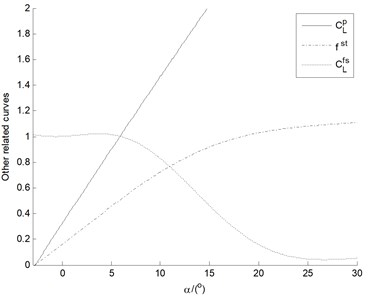
The nonlinear aerodynamic computation is implemented based on the three-fitted static elastic coefficients, which meanwhile can greatly reduce amount of calculation for various related parameters of the intermediate process and avoid aerodynamic strip decomposition along blade span. The three-fitted static elastic coefficients, and the other related intermediate parameters curves directly deduced by the fitted coefficients, are illustrated in Fig. 2.

Fig. 2a) The curves of the three-fitted static elastic coefficients and b) the other related intermediate parameters

a)

b)

4. Solution methodology

4.2. Assumption of structural damping

In order to accurately estimate the reliability of the blade motion, composite structural damping should be estimated. Whereas there is still no uniform structural damping estimation method. [17-20] investigates the structural damping of thin-walled composite one-cell beams based on modal damping ratio. Modal damping ratio of composite cross-section beam is defined as ratio of dissipated energy to maximum strain energy in the cycle of vibration. Based on research of [17], we investigate a structural analysis model which can determine the influences of different order modal damping factors for different structural and material parameters, and gives structural damping matrix based on Raleigh assumption [18]. To study the flexural vibration of the slender blade, based on modal damping factors above mentioned, another method is developed to compute structural damping as depicted in [19]. Structural damping from structural parts of blade section in Eq. (2-4) can be expressed in terms of an equivalent viscous damping matrix with 3×3$N$ as:

16a

$k_{11}={\oint }_{}\left(A-\frac{B^2}{C}\right)ds+\left\{{\left[{\oint }_{}\left(\frac{B}{C}\right)ds\right]}^2/{\oint }_{}\left(\frac{1}{C}\right)ds\right\},$
$k_{12}=\left[{\oint }_{}\left(\frac{B}{C}\right)ds/{\oint }_{}\left(\frac{1}{C}\right)ds\right]A_e,$
$k_{13}=-{\oint }_{}\left(A-\frac{B^2}{C}\right)yds-\left\{\left[{\oint }_{}\left(\frac{B}{C}\right)ds{\oint }_{}\left(\frac{B}{C}\right)yds\right]/{\oint }_{}\left(\frac{1}{C}\right)ds\right\},$
$k_{14}=-{\oint }_{}\left(A-\frac{B^2}{C}\right)xds-\left\{\left[{\oint }_{}\left(\frac{B}{C}\right)ds{\oint }_{}\left(\frac{B}{C}\right)xds\right]/{\oint }_{}\left(\frac{1}{C}\right)ds\right\},$
$k_{22}=\left[1/{\oint }_{}\left(\frac{1}{C}\right)ds\right]A_e^2,k_{23}=-\left[{\oint }_{}\left(\frac{B}{C}\right)yds/{\oint }_{}\left(\frac{1}{C}\right)ds\right]A_e,$
$k_{24}=-\left[{\oint }_{}\left(\frac{B}{C}\right)xds/{\oint }_{}\left(\frac{1}{C}\right)ds\right]A_e,$

16b

$k_{33}={\oint }_{}\left(A-\frac{B^2}{C}\right)y^{2}ds+\left\{{\left[{\oint }_{}\left(\frac{B}{C}\right)yds\right]}^2/{\oint }_{}\left(\frac{1}{C}\right)ds\right\},$
$k_{34}=-{\oint }_{}\left(A-\frac{B^2}{C}\right)xds-\left\{\left[{\oint }_{}\left(\frac{B}{C}\right)xds{\oint }_{}\left(\frac{B}{C}\right)yds\right]/{\oint }_{}\left(\frac{1}{C}\right)ds\right\},$
$k_{44}={\oint }_{}\left(A-\frac{B^2}{C}\right)x^{2}ds+\left\{{\left[{\oint }_{}\left(\frac{B}{C}\right)xds\right]}^2/{\oint }_{}\left(\frac{1}{C}\right)ds\right\},$
$A_e=\frac{1}{2}{\oint }_{}\left(x\frac{dy}{ds}-y\frac{dx}{ds}\right)ds.$

Meanwhile similar to the previous variation of the strain energy formulation, the variation of the dissipated energy of the cross section in terms of the strains ${\gamma }_{11}$ and ${\gamma }_{12}$can be deduced as [20]:

17

$\delta W_s={\oint }_{}\left[\begin{array}{ll}{\gamma }_{11}& {\gamma }_{12}\end{array}\right]\left[\begin{array}{ll}{A}_d\left(s\right)& B_d\left(s\right)\\ B_d\left(s\right)& C_d\left(s\right)\end{array}\right]\left[\begin{array}{l}{\gamma }_{11}\\ {\gamma }_{12}\end{array}\right]ds={\left[\mathrm{\delta }\mathrm{\Delta }\right]}^T{C}_C\left[\mathrm{\Delta }\right],$

where $C_C$ is 4×4 symmetric matrix with its components $c_{ij}$embodied. Hence the equivalent damping matrix can be similarly written as [20]:

18

$\stackrel{-}{C}=\left[\begin{array}{cccc}{c}_{11}{E}_{ij}& c_{12}{F}_{ij}& c_{13}{G}_{ij}& c_{14}{G}_{ij}\\ c_{12}{I}_{ij}& c_{22}{J}_{ij}& c_{23}{K}_{ij}& c_{24}{K}_{ij}\\ c_{13}{N}_{ij}& c_{23}{O}_{ij}& c_{33}{P}_{ij}& c_{34}{P}_{ij}\\ c_{14}{N}_{ij}& c_{24}{O}_{ij}& c_{34}{P}_{ij}& c_{44}{P}_{ij}\end{array}\right],$

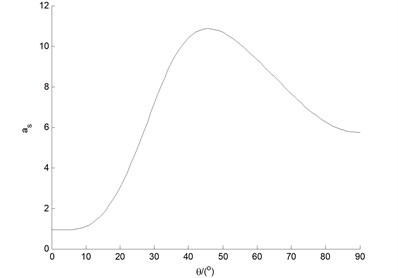
where the expressions of $c_{ij}$ are similar to those of $k_{ij}$, but the terms $A\left(s\right)$, $B\left(s\right)$, and $C\left(s\right)$ in $k_{ij}$ should be replaced by the equivalent parameter terms $A_d\left(s\right)$, $B_d\left(s\right)$, and $C_d\left(s\right)$ in $c_{ij}$, respectively. The expressions of $A_d\left(s\right)$, $B_d\left(s\right)$, and $C_d\left(s\right)$ can be found in [20].

Damping parameter factors ($a_s$) are illustrated with different ply angles ranging from 0°-90° in Fig. 3.

Fig. 3as as a function of ply angles ranging from 0°-90°

Integrating structural damping $C_s$ into Eq. (15) and carrying out the indicated variations and the required integration in Galerkin method, result in the matrix equations governing the system motion for blade tip as follows:

19

$M_M\ddot{X}+C_{SM}\dot{X}+K_{M}X=Q_M,$

with total 3$N$×3$N$ damping matrix $C_{SM}$:

20

$C_{SM}=C_M+{\left[\begin{array}{lll}\int C_{s11}{y}_{j}dz& \int C_{s12}{y}_{j}dz& \int C_{s13}{y}_{j}dz\\ \int C_{s21}{x}_{j}dz& \int C_{s22}{x}_{j}dz& \int C_{s23}{x}_{j}dz\\ \int C_{s31}{s}_{j}dz& \int C_{s32}{s}_{j}dz& \int C_{s33}{s}_{j}dz\end{array}\right]}_{3N\times 3N}.$

4.3. LQC control

In order to realize aeroelastic control for aeroelastic system Eq. (8), defining the state vector $Y={\left[X^T,{\dot{X}}^T\right]}^T$ and adjoining the identity equation $\dot{X}=\dot{X}$, Eq. (7) can be converted to the state space expression:

21

$\left\{\begin{array}{l}\dot{Y}=AY+Bu,\\ Y_o=CY+Du.\end{array}\right.$

The LQC controller is often used to analyze vibration control of rotating composite beam, one example is linear quadratic Regulator (LQR). An advantage of LQR controller is that it provides a systematic way of computing the state feedback control gain matrix $K$ of of the optimal control vector, so as to minimize the performance index [22]:

22

$J={\int }_0^{\propto }(Y^{T}QY+u^{T}Ru)dt,$

where 𝑄 and 𝑅 are the weighting matrices of system outputs and control inputs, respectively, with control signal set as:

23

$u^{*}=-KY\left(t\right)=-R^{-1}{B}^{T}PY\left(t\right).$

Herein, $P$ is a real symmetric matrix, satisfies the Riccati equation:

24

$PA+A^{T}P-PB{R}^{-1}{B}^{T}P+Q=0.$

The controlled state equation of the closed loop system [23] with state feedback is obtained as:

25

$\left\{\begin{array}{l}\dot{Y}=\left(A-BK\right)Y+Bu,\\ Y_o=\left(C-DK\right)Y+Du.\end{array}\right.$

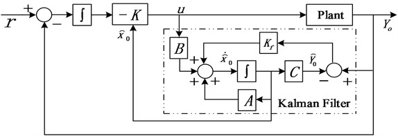
In order to suppress the too large initial vibration amplitude in LQR process, another LQC controller, the conventional linear quadratic Gaussian (LQG) controller is used to stabilize the displacements [24]. It consists of first determining the optimal control $K$ to a deterministic LQR problem, the second step to find an optimal estimate (of the state $Y$) given by a Kalman filter and independent of $Q$ and $R$, and the final connection of the Kalman filter and linear quadratic optimal gain $K$. However, the conventional LQG algorithm based on directly optimal control does not suppress the amplitude of the controller itself.

Here in order to suppress the too large amplitude of controller $K$, a special LQG controller with integral action for inverse response process is designed to decrease the amplitude of controller response [25]. LQG controller with integral action and reference input is illustrated in Fig. 4. The standard LQG design does not give a controller with integral action, so the plant here is augmented with an integrator before designing the state feedback regulator. A LQG servo-controller that uses the setpoint command $r$ and measurements $Y_0$to generate the control signal $u$ has integral action to ensure that the output $Y_0$ tracks the command $r$ with smaller controller amplitude. Here the control error $r-Y_0$ is integrated and the regulator $K$ is designed for the plant augmented with integrated states.

The Kalman filter has the structure of an ordinary state-estimator or observer characterized by:

26

${\stackrel{`}{\widehat{x}}}_0=A{\widehat{x}}_0+Bu+k_f\left(Y_0-C{\widehat{x}}_0\right),$

where $x_0$ is the state variable in LQG control with its optimal estimate being ${\stackrel{`}{\widehat{x}}}_0$; the optimal choice of $K_f$ minimizes $E\left\{\right[x_0-{\widehat{x}}_0{]}^T[x_0-{\widehat{x}}_0]\}$, which is independent of constant power spectral density matrices $W$ and $V$ in Gaussian stochastic noise processes and given by:

27

$K_f=Y_x{C}^T{V}^{-1},$

where $Y_x$ is the unique positive-semidefinite solution of the algebraic Riccati equation:

28

$Y_x{A}^T+A{Y}_x-Y_x{C}^T{V}^{-1}C{Y}_x+W=0.$

Fig. 4LQG controller with integral action and reference input

5. Results and discussions

Aeroelastic stability analysis can be implemented by time domain responses of Eqs. (9-10). Influences of ply angles and pitch angles on aeroelastic stability are investigated. The obvious effects of LQR and LQG controllers are demonstrated by vibration suppression for divergent cases.

5.1. Influences of ply angles and pitch angles on aeroelastic stability

Generally, with the range of 30°-60° of both ply angles and pitch angles, good aeroelastic stability of wind turbine blade can be obtained [18, 26]. Some cases intended to highlight the effects of ply angles and pitch angles under condition of $U=$5 m/s are presented.

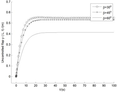
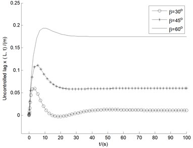
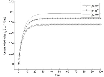
Fig. 5-6 show the uncontrolled blade tip responses of flap bending $y\left(L,t\right)$, lag bending $x\left(L,t\right)$, and twist ${\theta }_z\left(L,t\right)$, for ply angles ($\theta$) and pitch angles ($\beta$) in the range of 0°-90°, respectively. It is noticed from Fig. 5 that for all the three displacements within 40 s time, the amplitude of the vibration of $\theta =$30° quickly decreases in the state of convergence, and stabilizes at a lower numerical point. Comprehensive evaluation being from Fig. 6, it can be seen that the performance of $\beta =$45° is in the middle of all pitch angle instances, with all the three displacements convergent, and with moderate amplitudes after 25 s or so. Hence the follow-up study for stability analysis and control of divergent cases will take the fixed angles of $\theta =$30° and $\beta =$45°.

Fig. 5The responses of bending (y), bending (x), and twist (θz), for ply angles in the range of 0°-90°

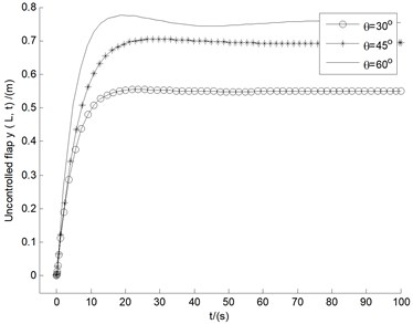
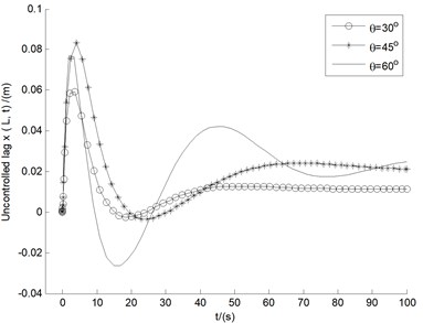
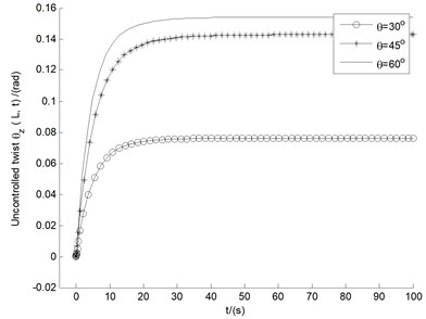
Fig. 6The responses of bending (y), bending (x), and twist (θz), for pitch angles in the range of 0°-90°

5.2. Influences of LQR control on aeroelastic stability

5.2.1. Influences of LQR control based on divergent cases

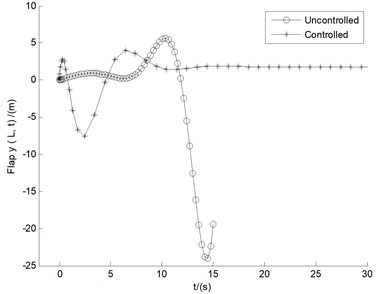
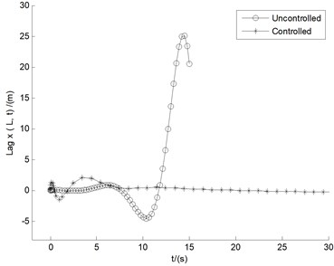
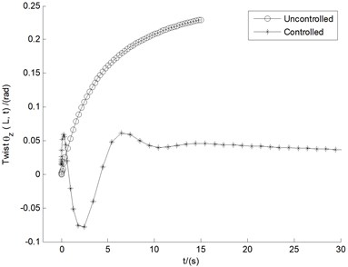
Fig. 7 shows the controlled responses of the three motions by LQR controller under $U=$10 m/s based on basic angles setting mentioned above. It shows that the three uncontrolled displacements, $y\left(L,t\right)$, $x\left(L,t\right)$, and ${\theta }_z\left(L,t\right)$, all show divergent states, with the amplitude of the vibration quickly exceeding the length of the blade $L=$15 m within time 15 s. Also in contrast with uncontrolled cases, the displacements controlled by LQR controller are of more advantages from the viewpoint of amplitude suppression. It can also be seen that the controlled flutter amplitudes of all the three motions decrease rapidly with the change of time, and tend to be steady within 15 s with tiny displacement deflection. It demonstrates apparent aeroelastic control effect of LQR controller on divergent aeroelastc instability.

In order to test such a LQR controller can be commonly used. Another divergent case of $U=$15 m/s is investigated in Fig. 8. Compared with the uncontrolled case of $U=$10 m/s, uncontrolled displacements especially for flap and lag motions under $U=$ 15 m/s, have a larger divergence, with the vibration amplitude more than the length of the blade within 3 s time. Also, Fig. 8 displays the amplitudes of LQR control for the three motions. It is obviously demonstrated the same conclusion as Fig. 7, namely that, the influences of LQR control on divergent cases are apparent.

Fig. 7Controlled responses of the three motions under U= 10 m/s

5.2.2. Analytical proof of the stability of LQR controller

The effectiveness of the stability analysis by LQR controller can be confirmed by eigenvalue analysis for homogeneous equation systems (only concerning the characteristic matrices of $A$ and $A-BK$ in Eqs. (21, 25), respectively) defined in state-space for $U=$ 10 m/s and $U=$ 15 m/s, respectively. Table 2-3 show comparisons of real parts of eigenvalues under uncontrolled cases and those controlled by LQR for $U=$10 m/s and $U=$ 15 m/s, respectively. If real parts of all the eigenvalues of the aeroelastic system are negative, the system is significantly stable. Furthermore, if the real parts of eigenvalues are arranged in order from large to small and named in order as Eig1, Eig2, Eig3, etc. (Note that the real parts are characterized by a total of thirty data, with only the first eight data listed in Table), the maximum aeroelastic instability might be decided. So, stability rules influenced by LQR controller might be clarified by comparison of corresponding eigenvalue pairs.

It can be seen from Tables 2-3 that the homogeneous equation system obtained by control of LQR controller is stable, with all the Real-parts of eigenvalues being less than zeros. Compared with the controlled system, the Real-parts of some characteristic values of the uncontrolled system are greater than zeros, which means that the uncontrolled system is not stable. The maximum value of Real-parts of uncontrolled system in Table 2 is 0.4278, with the maximum value of Real-parts of controlled system being –0.0285. We can get very similar stability conclusions in Table3 with $U=$15 m/s. The maximum value of Real-parts of uncontrolled system in Table3 is 2.7322, with the maximum value of Real-parts of controlled system being –0.1403. Moreover, for the comparison of every corresponding eigenvalue pair, the value under controlled situation is always less than that under uncontrolled situation, which means the excellent stability of the proposed LQR controller.

The stability conclusions from eigenvalue analysis in Tables 2-3 are in qualitative agreement with those from time responses in Figs. 7-8. It should be stated that the systems of Eqs. (21, 25) all are forced systems; compared with the stability conclusions from responses analysis of the forced systems, the stability conclusions from eigenvalues analysis of the homogeneous systems are more conservative.

Fig. 8Controlled responses of the three motions under U= 15 m/s

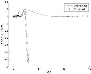
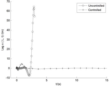
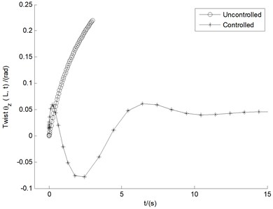
Table 2Comparisons of real parts under uncontrolled cases and those controlled by LQR for U= 10 m/s

$U=$10m/s	Eig1	Eig2	Eig3	Eig4	Eig5	Eig6	Eig7	Eig8
Uncontrolled	0.4278	–0.0272	–0.1397	–0.1402	–0.1405	–0.1407	–0.1415	–0.1454
Controlled	–0.0285	–0.1397	–0.1402	–0.1405	–0.1407	–0.1416	–0.1451	–0.1484

Table 3Comparisons of real parts under uncontrolled cases and those controlled by LQR for U= 15 m/s

$U=$15 m/s	Eig1	Eig2	Eig3	Eig4	Eig5	Eig6	Eig7	Eig8
Uncontrolled	2.7322	0.4279	–0.1403	–0.1414	–0.1421	–0.1425	–0.1445	–0.1532
Controlled	–0.1403	–0.1414	–0.1421	–0.1426	–0.1447	–0.1525	–0.1604	–0.1853

5.3. Influences of LQG control on divergent cases based on integral action for inverse response process

In view of the real-time implementation of LQR control, controller amplitudes of state $Y$ should be kept within a certain range to avoid hardware damage problems. Fig. 9(a) shows the constant LQR controller amplitudes of 30 (6$N$) state variables $Y$ in the divergent case of $U=$15 m/s in section 5.2.1. Notice that the horizontal coordinate values are represented by 30 state variables in turn. The order of magnitude of controller amplitudes reaches an incredible degree, so it is difficult to achieve in controller hardware design. Especially for seventh to tenth state variables, which imply the displacements of lag motion, the huge amplitude values also indicate that it is difficult to realize the flutter suppression for lag displacements.

Fig. 9(b) depicts LQG controller amplitudes in the divergent case of $U=$15 m/s as a function of time. For the three different motions, the amplitude values of the three controllers all are small, each stable at a very small value, which indicates the feasibility of real-time operation.

Fig. 9a) The constant LQR controller amplitudes of 30 (6N) state variables Y, b) and LQG controller amplitudes as function of time, in the divergent case of U= 15 m/s, respectively

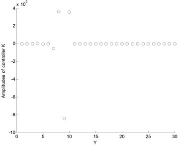
a) LQR

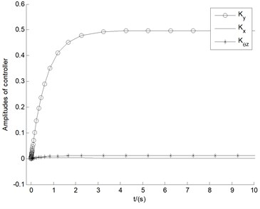
b) LQG

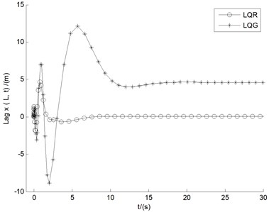
In Fig. 10(a-c), the control effects of both LQR and LQG in the divergent case of $U=$15 m/s are involved, where the comparison of the three controlled displacements is indicated. In contradistinction with the trends occurring in LQR control, the results of LQG are stable in larger numerical values with longer steady state time, which means that the reduction of the amplitude of the controller is accompanied by the attenuation of the control performance. In Fig. 10(d), the real parts deviations of the first eight largest eigenvalues (similar to Tables 2-3) between LQR and LQG are illustrated. The very small deviation data show relatively close control performance between LQR and LQG, especially the first four decisive values (Eig4-Eig1) are very close, which demonstrates the stability rules coincide with those in Fig. 10(a-c) obtained via the numerical responses of the three displacements.

Anyway, Fig. 9-10 show an expected conclusion, namely that for stability analysis of stall flutter, LQR and LQG, each can play an important role in enhancing the vibration behavior of the structure.

Fig. 10Effects of both LQR and LQG in the divergent case of U= 15 m/s

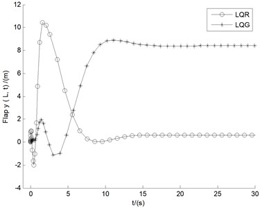
a) Flap

b) Lag

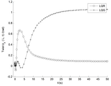
c) Twist

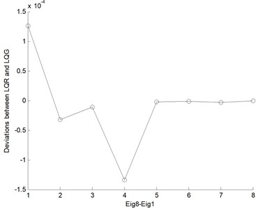
d) Real parts deviations

6. Conclusions

Bending-bending-twist stall flutter behavior and linear quadratic control of wind turbine blade are investigated. The analytical study and numerical illustrations reveal the results:

1) Vibration behavior is investigated and discussed based on symmetric layup configuration. The nonlinear aerodynamic forces are characterized by B-L model based on fitted static aeroelastic coefficients. Stall flutter and aeroelastic stability are analyzed based on ply angles and pitch angles. Aeroelastic control is carried out by LQR and LQG controllers.

2) The method of fitting aeroelastic coefficients in B-L model can greatly reduce the complexity of processing, avoid the nonlinear aerodynamic strip decomposition and reduce the number of equations, and realize Galerkin method directly through the integral action along the blade span.

3) The obvious effect of LQR controller is demonstrated by vibration suppression for divergent cases, with validation implemented by eigenvalue analysis. In order to avoid excessive controller amplitude in LQR, LQG control in applied. However, the reduction of the controller amplitude is accompanied by the attenuation of the control performance in LQG, with larger time response amplitude and longer steady state time obtained.

4) Control performance of LQG based on integral action for inverse response process is illustrated, accompanied by excellent real-time controller amplitude. In contrast to responses in the divergent cases, the effectiveness of LQR and LQG is reflected in both decreasing amplitudes and reducing steady state time.