Acousto-ultrasonic analysis of defects in composite specimens used in transportation domain

1. Introduction

Recently, the transportation industry has been changing direction by substantially reducing the use of metal parts paving the way towards the use of composite materials parts [1]. Composites possess certain properties including strength, stiffness and reduced weight [2]; thus, their emergence in the aviation and transport industry in general is not a surprise. These characteristics constitute composite materials an appropriate solution for other modes of transportation such as the railway industry [3].

Although the railway is considered to be among the most environmentally friendly means of transportation, there is still room for improvement. Further decrease in environmental impact by utilizing new technologies at the inception of product design and development needs to be taken into account. An additional contemplation is the energy impact of composite-carbodies due to their weightless property [4]. Reducing the rail car-body mass, which often comprises heavy metal parts, is the necessary procedure for the next generation of trains as to introduce energy saving. A primary action to reduce weight could be the substitution of steel with composite components while maintaining safety [5].

Non-Destructive Testing (NDT) and Structural Health Monitoring (SHM) inspect and monitor the state of critical modes and infrastructures respectively, whose problematic states may be repaired in a costly manner and can even put lives in jeopardy [6-9]. NDT is a technique that specialises in the inspection of structures in order to recognise and locate flaws, non-homogeneity in microstructures, delamination, deformation and others [10]. A SHM system comprises an array of connected sensors, which gather the respective data during the service life of the equipment and infrastructure continuously. SHM systems are employed to locate, discover and identify occurred damage or state of deterioration that typically takes place over the service life [11].

Acousto-ultrasonics (AU) are closely related to the methodology of Acoustic Emission (AE). AU may be distinguished as AE simulated with or assisted by ultrasonic sources. The key difference between AU and AE methods can be located in the stress waves, whereby the AE method depends on structural loading thereby exciting instant and spontaneous stress waves. On the other hand, in AU the ultrasonic waves are induced by external transducers [12].

AE constitute a significant methodology in the SHM research [13]. AE, along with the underlying technology of piezoelectric transducer mechanism (lead zirconate titanate PZT and relevant piezoelectric ceramics and crystal), has played an important role in the detection of failures in the transport industry. AE monitoring applications comprise aircraft material state monitoring, high speed train car-bodies, bridges and rail tracks [14-17].

AE, except from metal parts, can be employed for the characterisation of composite materials as defect-full. Structures made of composite material require their health assessed as well, since they are prone to defects, such as delamination, matrix crack, fiber-matrix debonding and fiber breakage [18]. The advantages of AE monitoring are more than enough and they are evident in the relevant literature [19-24]. Certain advantages of the AE methodology includes, real-time assessment with monitoring, cost-efficiency, early-stage and quick defect identification (predictive maintenance), distinguish between fault, high fault sensitivity and maintenance budgeting [25]. The nature of the AE monitoring allows assets to be inspected or monitored in a continuous manner and without terminating operations; thus, reducing downtime and enhancing productivity and shorter asset depreciation.

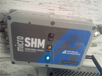
In this paper, we utilised the Mistras Micro-SHM (https://www.physicalacoustics.com/by-product/micro-shm-structural-health-monitoring-system/) system to perform three sets of experiments using composite material specimens and two different sensors, namely R6a and R15a. The first set of experiments consisted of the attenuation measurement of AE produced by Pencil Lead Breaks (PLB) indicating the impact of the reflection from its edges. The second experiment set consisted of three sub-experiments objective and its objective was to identify defects using two signal features; note that the initial experiment of the set was with no defect and the latter two with different defects introduced on the specimen. The significance of the experiment arises from the fact that the signal may suffer from reflections due to its small size. Finally, a new larger triangular-shape composite specimen was utilized in order to stress out the difference in the two signal features between the specimens, and thereof further investigation on the specimens is essential.

2. Experimental Procedure and Setup

The R15a and R6a sensors were used for the experiments. The R15a and R6a sensors are narrow band resonant sensor with a high sensitivity. Their main differences can be found in the operating specifications. In particular, the differences between the two sensors are given in the following table:

Furthermore, for the three sets of experiments, the settings of the Micro-SHM system parameters include a 2 Mega Samples per Second (MSPS) sampling rate, with 2k samples buffer depth. Moreover, an analog filter from 10kHz to 1MHz and a digital butterworth bandpass filter from 80kHz to 200kHz were set in order to prevent the inclusion of external noise; for example, instability of the researcher hand performing the PLB, as well as background noise. During the first experiments, a 200 mm length and 70 mm width specimen was used. In the second set, 200 mm length and 75 mm width specimens were employed. For the third experiment, we used a thinner and larger triangular-shape composite specimen with the PLB distance being larger than the length of the first two specimens. Note that these specimens are obtained by experts who will attempt to use them in train car bodies; as such experiments regarding their health and structural integrity are vital.

2.1. Experiment setup for attenuation

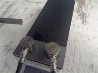
The first set of experiments was conducted in order to exhibit the device sensitivity using a small size specimen. In particular, measurements included the attenuation of AE produced by PLB using the R6a and R15a sensors. It has been proven in the literature [26] that a 0.5 mm pencil with 2H hardness can closely simulate the AE event produced from the specimen under strain. The specimens were two PREPEG (https://en.wikipedia.org/wiki/Pre-preg) and Polyethylene Terephthalate (PET (https://en.wikipedia.org/wiki/Polyethylene_terephthalate)) composite with the same dimensions but of 10 mm and 25 mm thickness respectively. Fig. 1 illustrates the experimental set-up and the wireless AE acquisition system.

Fig. 1a) Overview of the experimental layout with specimen and sensors, b) Mistras micro-SHM wireless AE acquisition system

a)

b)

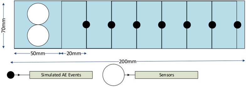
The specimen (70 mm width and 200 mm length) was mounted on top of triangular wedges through soft damping patches. Along the 200 mm side of the specimen, in the middle, a line was drawn with test points every 20 mm starting with a 50 mm distance from the left side of the specimen, where the sensor was placed (Fig. 2). Fig. 2 is a graphical representation of the experiment setup showing only the dimensions of the specimen and the distances between the sensors and the PLBs. A total of four PLBs were recorded on each test point.

Fig. 2Attenuation distance points of simulated ΑΕ events

2.2. Defect experiment setup

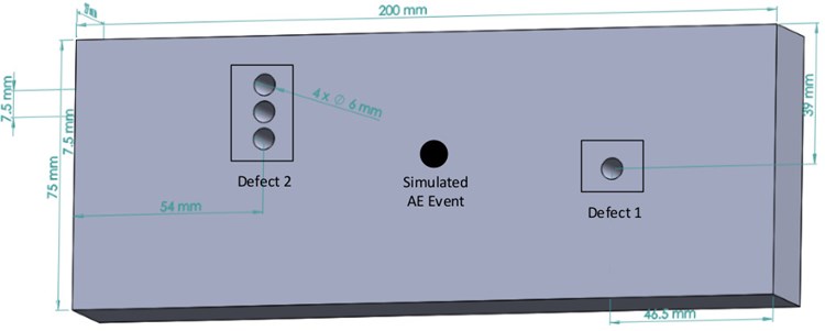
The defect identification experiment comprised the use of two identical specimens (75 mm width and 200 mm length). The first one was used in tact, in order to obtain readings of PLBs without defect. The twin specimen was pierced with one and three holes respectively along the specimen’s long side. Henceforth, for ease of explanation, the setup with the one hole is denoted as Defect 1 and the setup with the three holes as Defect 2 respectively. The PLBs responsible for the generation of the simulated AE event was conducted in the middle of the specimen with respect to the width and length of the specimen. The following three experiments were performed: i) Free-Defect using similar free of defect specimen ii) Defect 1 and iii) Defect 2, using a twin specimen. A 3D top layout for Defect 1 and Defect 2 topologies is presented in Fig. 3. The goal of the trials was to demonstrate the AE system capability to recognize defects that reside prior to the simulated AE event in the Line of Sight (LOS) with the sensor. Two sets of four PLBs were performed per experiment. The values that have been obtained come from the AEWin software, which accompanies the Micro-SHM system. Statistics produced by AEWin include the minimum, maximum and average values of several signal features for each of the four simulated AE trials. The average value of the ‘Amplitude’ and ‘PAC Energy’ were obtained per trial and were averaged to get the values shown in the results section. Henceforth, we will call the free of defects as specimen 1 and the twin specimen with the defects as specimen 2.

Fig. 3Model of defect experiment

3. Results

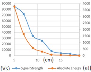
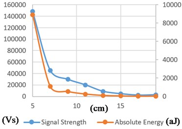
The following parameters ‘Duration, Amplitude’, ‘Average Signal Level’ (ASL), ‘Average Frequency’, ‘Reverberation Frequency’, ‘Initialisation Frequency’, ‘Signal Strength’ and ‘Absolute Energy’ [27] have been extracted in the attenuation experiments. Note that a number of other parameters could be used, offered by the Mistras Micro SHM system and software; however, our intention is to show the measurements taken from both sensors and both specimens.

Fig. 4Triangular-shape specimen with sensors and PLB position

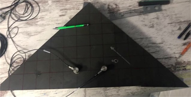
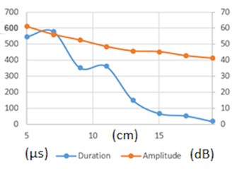
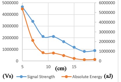
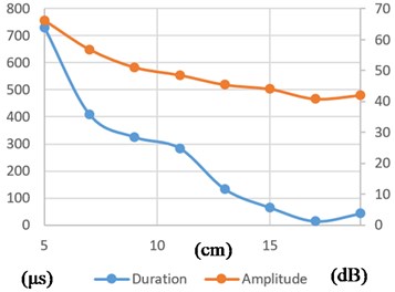
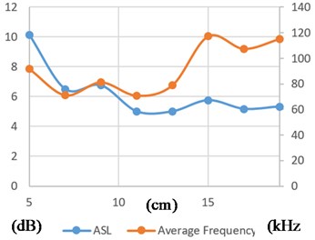
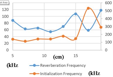
Fig. 5PREPEG+PEG with 10 mm thickness AE features sampled from 50 mm distance up to 190 mm for R15a sensor

a)

b)

c)

d)

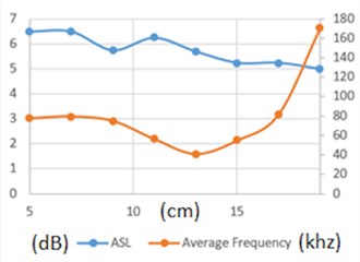
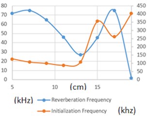
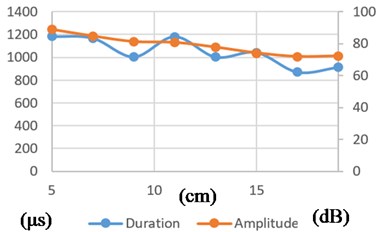
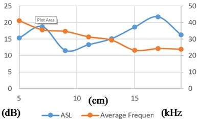
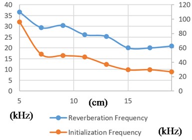
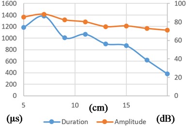
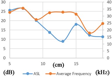
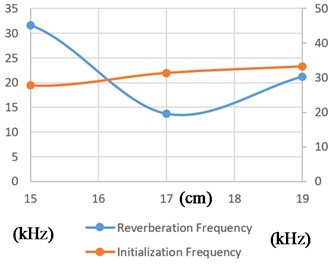
Some brief comments on Fig. 5 results. Duration (Fig. 5(a)) is defined as the time from the first threshold crossing to the end of the last threshold crossing of the AE signal from the AE Threshold (The Threshold Feature records the value of the Threshold at the time of an AE occurrence). The Amplitude is the maximum (positive or negative) AE signal excursion during an AE hit, measured in 20log scale (dB). It is clear that duration drops strongly as the point of failure moves away from the sensor. Of course the wave shape of duration waveform is attributed to the reflections from the specimen boundaries. In a less degree decrease was observed with the amplitude waveform. Moreover, as can be seen at Fig.5.d Average Signal Level (ASL) is a measure of the continuously varying and “averaged” amplitude of the AE signal and is measured in dB. The average frequency feature, reported in kHz, determines an average frequency over the entire AE hit. The ASL exhibits the usual attenuation over distance, and it can be noted that the drop is not substantial which makes the feature ideal for above 40 or 50 cm distant failure sources. The average frequency appears somewhat erratic for the long distances. This feature along with the Reverberation Frequency (Fig. 5(c)), which can be thought of as the “ring down” frequency since this is the average frequency determined after the peak of the AE waveform, and Initiation Frequency, which can be thought of as the “Rise Time” frequency (this feature calculates the average frequency during the portion of the waveform from initial threshold crossing to the peak of the AE waveform), all three features at long distances appear to have an erratic behaviour with high frequency values. This erratic behaviour is attributed to the fact that as the distance rises so does the attenuation and along with the fact that the R15a is high pass filter with resonance above 100 kHz results in high frequencies appear magnified in correlation to low frequencies at long distances.

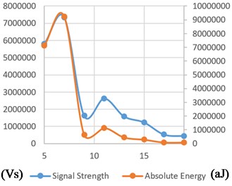
Finally at (Fig. 5(d)), the Signal Strength is mathematically defined as the Integral of the rectified voltage signal over the duration of the AE waveform packet, and Absolute Energy is a 6-byte value whose units are aJ (or attoJoules). They have a clear drop for distances far from the sensor, as was expected.

All these aforementioned features give a rich features space to describe various kinds of failures with various depth within the specimen and distance from the sensor.

Fig. 6PREPEG+PEG with 10mm thickness AE features sampled from 5cm distance up to 19 cm for R6a sensor (descriptions for a), b), c) and d) are the same as in Fig. 5)

a)

b)

c)

d)

Fig. 7PREPEG+PEG with 25mm thickness AE features sampled from 5cm distance up to 19 cm for R15a sensor (the descriptions for a), b), c) and d) are the same as in Fig. 5

a)

b)

c)

d)

Fig. 8PREPEG+PEG with 25 mm thickness AE features sampled from 5 cm distance up to 19 cm for R6a sensor (the descriptions for a), b), c) and d) are the same as in Fig. 5)

a)

b)

c)

d)

As a general observation, Figs. 5-8 show that high sensitivity is possible up to 300 mm because of composite damping. When it comes to longer distances, hit energy values are essential. The resolution that we may achieve in terms of detection distance can be more than 1 meter; however, in order for this to be possible, more and detailed experiments with composite specimen of larger size should be conducted, since the specimens 1 and 2 are quite small and are susceptible to vast edge reflections. Because of the sensitivity and nature and of AEs, also by selecting sensors with a frequency of resonance above 200 kHz, the use of this methodology is highly recommended for critical car body parts and joints.

During the defect experiments, the data that have been gathered compares the readings of the sensors when Free-Defect, Defect 1 and 2 were performed. We extracted the PAC Energy and amplitude metrics using the R15a sensor, presented in Table 2.

Energy count are higher when there is no defect in the composite plane.. This helps verify the correct functionality of the sensor R15a and the system as a whole, since the PAC Energy should be lost from the defect experiments in front of the sensors. We see a clear reduction of energy count in the Defect 2 experiment. To be more specific, we see a 0.63 units reduction in PAC energy for the Defect 1 experiment compared to the Free-Defect experiment. For the Defect 2 experiment we notice a 47 % reduction of PAC Energy compared with the Free-Defect composite.

Additionally, amplitude reduction was observed due to defects presence. In fact, this result was something we had expected since the amplitude is supposed to be larger in the Free-Defect experiment. Nevertheless, the amplitude difference between the Free-Defect and Defect 1 experiments is very small. This difference is easier to see with Defect 2. Particularly, the reduction values are 1.875 dB and 3.875 dB.

Thereon, we performed the same experiments with the R6a sensor. We can see the results of the amplitude and the PAC Energy in Table 3. Again we observe that the energy is lower with the presence of defects. The scale of measurements is different, which comes as a result of the differences in the sensors and the preamplifiers. There is a 11 % difference between the free of defect and the Defect 1 experiments. As for the Defect 2 experiment, it exhibits a 38 % reduction with the free of defect as a reference.

In the amplitude measurements with the sensor R6a sensor, initially, we observe greater values in the measurements. The average amplitude values show a reduction as well with the presence of defects. More specifically the experiments exhibit a reduction of 4.75 dB and 5.75 dB for the 1 and 3 holes experiments respectively.

The final experiment of this paper involved the use of the specimen 3, which is larger than specimens 1 and 2 utilised in the former experiments. We measured the amplitude and PAC Energy, incorporating both the R6a and R15a sensors. We provide the average values obtained in Table 4.

In terms of the R15a sensor, the results show that even though the distance of the PLB and the sensors is larger than the distance in the experiment with specimen 1, the amplitude and PAC energy is significantly higher. This can be implicitly derived from the maximum height of the former specimen and the PLB breaking point of specimen 3. In specimen 1, the average was 49.5 db, while this specimen exhibited 76 dB amplitude. Certainly, there is a significant difference in the PAC energy as well, where the value of the former specimen was 4, while the average value using specimen 3, showed 118.6.

The values of the R6a sensor showed a large difference in the PAC energy and a moderate difference in the amplitude values. Specifically, using specimen 1 the PAC energy is 252.63 while using specimen 3 the value climbs to 823. Moreover, the amplitude value using specimen 1 is 79 dB, while using specimen 3 the amplitude reaches 91.10 dB.

We believe that different specimen material provided this difference. The specimen 3 is more stiff and denser compared to specimen 1, which is smaller and lighter, with additional dumping coming from the foam between the upper and lower composite reinforcement sheets.

4. Conclusions

The results presented in this paper were derived from an initial test of a small composite specimen by the use of two AE sensors, namely the R6a and the R15a sensors. To begin with, we measured the attenuation in a two composite material specimens of different thickness, using the two sensors, showing the influence of the reflection from its edges. It was shown that there is damping with the increase of distance from 50 mm to 190 mm. Further, we carried out experiments with two configurations of defects, as well as no defects using the two available sensors. It was determined that the defects could be identified by the AE sensors, since the energy count and the amplitude are reduced in the presence of defects.

Moreover, we utilized a larger specimen and we placed the sensors further away from the PLB to check the aforementioned features. The results using the two sensors showed that even though the distance is higher, the amplitude and PAC energy using specimen 3 was higher than when using specimen 1. This might be the case due to the material of the composite. In any case, the difference between the different composite-material specimens need to be further investigated. In particular, the specimen 3 needs to be assessed in more details before reaching a concrete conclusion, regarding the difference in the metrics obtained.

This work is purely experimental and it does not address the SHM of the composite in a theoretical manner; however, it provides experimental data obtained by real measurements on composite materials that will be used in the railway domain. Prediction of the data obtained are considered as future work. Moreover, defects in the new specimen need to be introduced, in order to investigate whether they will be identified by the equipment.