Analysis of the vehicle: applying finite element method of 3D data

1. Introduction

In a broad sense, computer-aided software systems that allow engineering studies to be carried out in a virtual environment with computer software, testing designs in a virtual environment, and design verification studies in a virtual environment have become more and more common [1].

The first development of the CAD system began in the late 1950s with the design of the DAC (Design Automated by Computer) system. It was the first computer graphics package to allow user interaction with designs and pioneered the beginning of the CAD system and then The Finite Element Method was first developed in 1956 for the stress analysis of airframes and started to be used in solving engineering problems. Fundamental logic is a numerical method used to solve problems that can be expressed in partial differential equations or formulated as functional minimization. For a structural simulation, FEM is very helpful for minimizing weight, materials and costs with the Finite Element Method, it is applied to systems with complex boundary conditions, systems with irregular geometry, steady state, time dependent and eigenvalue problems, linear and nonlinear problems [2, 3].

Along with the developments in the field of Computer Aided Design (CAD) and Finite Element Method, in the field of Vehicle Collision Simulation in the 1970s, car accident events were tried to be simulated. However, just like the more detailed finite element models, only the structural geometry and basic material properties need to be defined as an input to construct the numerical model. LS-DYNA, which was developed for Finite Element Analysis, was started to be developed in 1976 for use in areas such as the Finite Element Analysis (FEA) program, such as automobiles and aviation [4-6].

When the simulation of the accidental collision of a military fighter was introduced in 1978, automakers used this technology to simulate devastating car crash tests. In the following years, automakers produced more complex collision simulation studies, simulating the collision behavior of individual car body components, bodies for component assemblies. The results recreated the front effect of the passenger car structure, and the engineers were able to make effective and progressive improvements in the crash behavior of the analyzed car body structure [7, 8].

Technology continued to evolve with the rise of industry-standard computers in the 1980s, and the first program to allow 3D design emerged. With this development, the simple parts planned to be made have started to be displayed in the computer environment, and over the years, many design programs that are actively used in the engineering design processes have emerged over the years. Along with the developing technologies, many CAD programs were produced after the 1990s [9, 10].

In the 2020s, many studies have been carried out with the Finite Element Method and programs such as Computer Aided Design (CAE), FEA (Finite Element Analysis) and Ls-DYNA continue to be actively used today. This allowed the tests to be performed quickly and inexpensively on a computer, allowing for optimization of the design before an actual prototype of the vehicle was produced. Using a simulation, it solves problems and presents solutions to problems that may be nearly impossible before spending time and money on a real crash test [11, 12].

In Finite Element Analysis in order to obtain parameters in the mathematical calculation process, the design must have a drawn geometry (CAD) in the virtual environment, and then material information and analysis conditions (boundary conditions). As a result, for the current model, after the determination of the model, the following material processes and volume, solid and surface (shell) operations are applied [13, 14]. And in the Finite element method, no nodal point on the design is independent of each other. The nodes connected by the elements are thus connected to each other mathematically. As a result, the principle of Virtual Working is equal to Total internal virtual working and Total external (external) virtual working area (in the case of Harmonious equilibrium) and in this way it is mathematically progressed [15, 16].

Vehicle simulations are important both in vehicle design and in minimizing the damage caused by the use of vehicles. The accident scenarios of the vehicles analyzed with these simulations are obtained as data and can provide us with important data with applications such as machine learning and artificial intelligence. These data can present us how we can take precautions in active or passive safety systems before the design of vehicles. For example, since the collision analysis of a vehicle produced in valuation systems such as Euro NCAP is performed, it is necessary to go back to the design. However, collision behaviors can be predicted before they are produced by collision analysis in the simulation environment of the designed vehicle.

In this study, the logic of working with a mathematical approach for Finite Elements of a vehicle data with fasteners and material data is explained. Thus, the Finite Element Method will enable vehicle collision and different tests for Finite Element analysis.

2. Methods

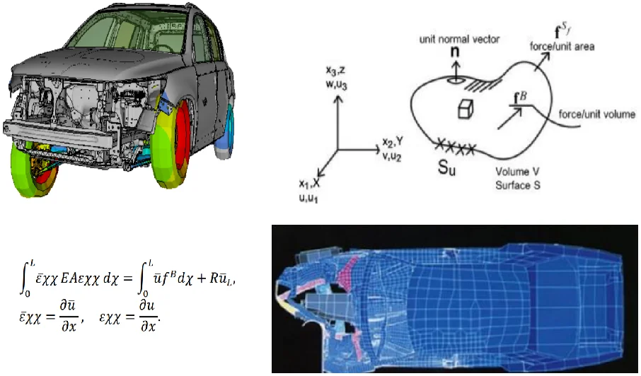
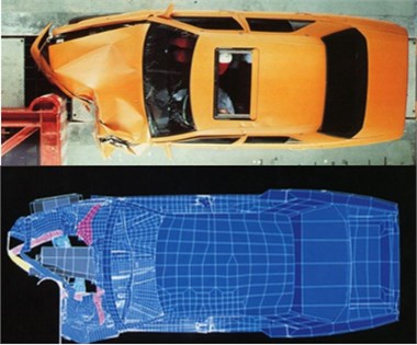
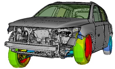
FEA is a numerical method used to predict how a part or assembly will behave under certain conditions. It is used as the basis for modern simulation software and helps engineers find weak spots in their designs. As shown in the Fig. 1, Collision model applied in the real and analysis environment.

FEA is a numerical method used to predict how a part or assembly will behave under certain conditions. It is used as the basis for modern simulation software and helps engineers find weak spots in their designs. In the automotive design process, the durability evaluations of components as a result of experimental evaluation are time-consuming and expensive. For this reason, analytical approaches that include a limited number of component verification tests have attracted more attention, and the test process is applied considering the conditions and criteria that the current system will work under in the FEA analysis process.

In this study, the determination of the vehicle collision model applied with the finite element method according to the desired analysis and the mathematical approach of the finite element analysis are explained.

Fig. 1Collision model applied in the real and analysis environment

2.1. Analysis applied in finite element analysis

– During the implementation of Finite Element Analysis, steps are applied in line with the purpose of the analysis:

– Modal Analysis (Studies on subjects such as Natural Frequency, vibration, noise).

– Temporary Dynamic Analysis (Studies on issues such as physical displacement and velocity of the system in response to events).

– Bending Analysis (Bending cases and post-bending issues are studied due to the carried loads).

– Contact Analysis (We are working on contact and fatigue analysis).

In the Finite Element Analysis process, different tests are applied for different analysis processes.

2.1.1. Durability analysis

Durability analysis evaluates the failure against repeated simple or complex loading. Therefore, the purpose of stress analysis is to obtain the full three-dimensional stress and strain distributions in a potential fault region, thus facilitating fatigue life estimates. It also predicts whether the component will be susceptible to breakage, distortion, bending, fatigue, or wear and tear when subjected to stress. While performing strength analysis, stress and strain values are required, so triangle element should not be used, therefore FEA model should contain only quadrilateral or hexagonal elements. When performing collision analysis, both triangular and quadruple mixed lattices can be used.

2.1.2. Noise, vibration and harshness analysis

Noise, vibration and harshness (NVH) is defined as the study and modification of the noise and vibration characteristics of vehicles, especially cars and trucks. Also, Interior NVH deals with noise and vibration experienced by cabin occupants, while exterior NVH is largely related to vehicle-emitted noise and includes continuous noise testing.

In Fig. 2, the noise, vibration and hardness studies are carried out on a vehicle model together with the NVH test and different forms of application are offered together with the NVH tests:

– Modal (structural) analysis;

– Frequency response analysis;

– Powertrains;

– It includes damping simulation processes.

Fig. 2Model with noise, vibration and harshness applied

2.2. Finite element method mathematical approach

For any input y applied in any system, the system response $\chi$ is shown using the scaling factor $\mathbf{K}$ as Eq. (1):

1

$\mathbf{K}\times \chi =y.$

For this equation, $\mathbf{K}$ is the spring stiffness, $\chi$ is the spring displacement, and $\mathbf{y}$ is the applied force. For any system, the above equation can be written as Eq. (2):

2

$\left[\mathbf{K}\right]\left\{\chi \right\}=\left\{y\right\},$

where $\left\{\chi \right\}$ displacements, temperatures, etc. $\left\{y\right\}$ can be a force, flow and etc. The matrix $\left[\mathbf{K}\right]$ can be regarded as a coefficient or more commonly as a stiffness matrix.

For the response $\left\{\chi \right\}=\left\{\alpha \right\}$, if the applied input is $\left\{y\right\}=\mathbf{L}\left\{\alpha \right\}$, they are known as eigenvalues and the system’s response $\left\{\alpha \right\}$, are also known as eigenvectors corresponding to the eigenvalue $\mathbf{L}$. The formula used in dynamic calculations is as Eq. (3):

3

$\left[\mathbf{M}\right]\left\{\ddot{u}\right\}+\left[\mathbf{C}\right]\left\{\dot{u}\right\}+\left[\mathbf{K}\right]\left\{u\right\}=\left\{\mathbf{F}\right\}.$

In the Eq. (3), formula, $\left[\mathbf{M}\right]$ is the mass matrix, $\left[\mathbf{C}\right]$ is the damping matrix, $\left[\mathbf{K}\right]$ is the stiffness matrix. $\left\{\ddot{u}\right\}$ (m/s²), $\left\{\dot{u}\right\}$ and $\left\{u\right\}$ are acceleration, velocity and displacement vectors and $\left\{\mathbf{F}\right\}$ is the force vector. Beside these, these vectors are functions of time.

To obtain these parameters, the design must have a drawn geometry (CAD) in the virtual environment, and then material information and analysis conditions (boundary conditions). As a result, after the determination of the model for the current model, the following material processes and volume, solid and shell processes are applied as in the Fig. 3.

Fig. 3Finite element analysis material and element types structure

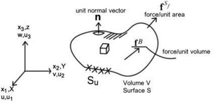
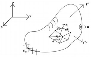
We consider a data/model and define the following quantities:

${–s}_u$: The surface where displacements and velocities are accepted;

${–s}_f$: Surface of applied forces;

$–f^{S}f$: Forces per unit surface;

${–f}^B$: Forces per unit volume.

$–Su\cup Sf=S$; $Sf\cap Su=\varnothing$.

External loads $f^B$ are applied to the volume of the body and external loads $f^{S}f$ to the surface of the body. The volume of the body is solved for the response of the body, given the boundary conditions at the surface (analysis scenario), the volume and the applied loads on the surface, and the material data.

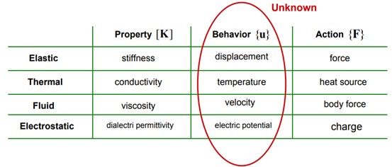
Considering the System Geometry ($V$, $Su$, $Sf$), charges ($f^B,f^{S}f$) and material laws are as follows:

– Displacements $u$, $v$, $w$ or ($u_1$, $u_2$, $u_3$).

– Stress – Strain:

4

$\left[\mathbf{K}\right]\left\{u\right\}=\left\{\mathbf{F}\right\}\Rightarrow \left\{u\right\}={\left[\mathbf{K}\right]}^{-1}\left\{\mathbf{F}\right\}.$

In the Eq. (4), formula, $\left[\mathbf{K}\right]$ is the property, $\left\{u\right\}$ is the behavior, $\left\{\mathbf{F}\right\}$ is the action.

Fig. 4Finite element analysis virtual displacement table

The formula specified for $\tau \chi \chi =E\frac{du}{d\chi }$ is used for Stress – Strain. In Virtual Displacement Principle, Real stresses ($C\epsilon$) are in equilibrium with external forces ($f^{S}f$,$f^B$):

5

$\frac{EA}{L}$$u$$\mathbf{F}$

6

$\mathbf{K}\times U=\mathbf{F}.$

As a of result formula in the Eq. (6), is used for Virtual displacement. Here it describes the displacement that occurs after a force applied to an existing body.

For the exact solution for stability in virtual displacements ($u\chi$) in the Eq. (7):

7

$\left(EA\frac{d^{2}u}{d{x}^2}+f^B\right)\delta u\left(\chi \right)=0.$

(Internal Virtual Work) = (External Virtual Work) + Virtual work due to boundary forces in the Eq. (8):

8

${\int }_0^L\frac{d\delta u}{d\chi }EA\frac{du}{d\chi }d\chi ={\int }_0^L{f}^B\delta ud\chi +R\delta u,$

where $\frac{d\delta u}{d\chi }$ is imaginary stresses, $\frac{du}{d\chi }$ is real stresses, and $\delta u$ is imaginary displacements. When the external forces are not known on $\delta u=$ 0 to calculate virtual work.

3. Conclusion

As a result of Virtual Working principle = Total internal virtual working and Total external virtual working area is equal in the Eq. (10):

The meshing process is to reduce a design consisting of infinite points to finite points in the most ideal way. Each point that occurs is called a node. For each node its own equation of motion is created by providing three conditions:

$–$Equivalence: in solids, $\mathbf{F}$ (N) =$m$ (kg) × $a$ (m/s²) for conservation of momentum in fluids;

$–$ Suitability: For continuity and boundary conditions;

$–$ Structural Connections: Used for Stress / Strain law.

In the finite element method, no node on the design is independent of each other. The nodes connected by the elements are thus connected to each other mathematically. The equation of motion for each point at each degree of freedom is combined to form an equation of motion for the entire design.

The equation of motion for each point at each degree of freedom is combined to form an equation of motion for the entire design.

Degrees of freedom: In general conditions, an independent point in space can move in 6 different ways. Of these, 3 are spherical (on the $X$, $Y$, and $Z$ axes), and 3 are local (around the $x$, $y$, and $z$ axes). The ability of a point to move is called the degree of freedom. In finite elements, the degrees of freedom of the points connected by the elements are also limited as shown in the Fig. 5.

Fig. 5Table finite element analysis degrees of freedom

$\tau ij,j+fiB=0$ in V → Equilibrium conditions.

$\tau ijnj=f{i}^{S_f}$ on $s_f$ → Equilibrium conditions.

$u_{i}lSu$ = $u{i}^{S_u}$ → Eligibility conditions.

$\tau ij=f\left(\epsilon kl\right)$ → Stress – Strain connection.

In the Eq. (11), continuity and boundary conditions according to degrees of freedom, connections and equivalence data.

In this study, analysis and mesh structures are explained according to the type of analysis (such as vibration, displacement, velocity and fatigue analysis) to be done with the Finite Element method.

In addition, the mathematical structure of the finite element analysis and the displacements in the structure to be analyzed, the applied forces, the forces at the unit volume and the surface, and the virtual working principle are explained.

Continuity and boundary conditions, structural connection and equivalence data are mentioned in the meshing process in the analysis data.