Abstract
Bearings are integral components of rotating machinery and their failure tends to be a catastrophic failure of the machine. Poincare Maps are used to detect bearing failures using the concept of non-linear dynamics. Each time-domain vibration signature array has its own Poincare Map over a period of time. Fast Fourier Transform (FFT) is a method of analysing the frequency plots of a bearing signature. Convolutional Neural Networks (CNN) process the bearing Continuous Wavelet Transform images and provide the Remaining Useful Life (RUL) of the bearing. The Poincare Maps and FFT plots are used to diagnose the type and location of the fault in the bearing, whereas the CNN helps to provide the fraction of Remaining Useful Life. The study concludes that a combination of Poincare Maps, FFT analysis and Convolutional Neural Networks constitutes a robust and precise method of monitoring bearing conditions.
Highlights
- Non-periodic nature of the motion of spin elements cannot be detected using frequency spectrum analysis. Poincare Maps of vibration signature arrays of large numbers of data points resolve this issue.
- The Poincare Maps generated from the vibration accelerometer data can be reliably used to diagnose the approximate location and severity of the defect.
- Poincare Map describes the location of the defect relatively approximately with reference to the shaft position.
- Using CNN to predict the fraction of RUL gives a very accurate measure of the Remaining Useful Life of a bearing. The research on RUL of the bearings was conducted using the FEMTO dataset.
- Using CWT and CNN to predict the fraction of Remaining Useful Life gave a 94.00 % median accuracy and a mean accuracy of 93.14 % on the test sets.
- The methodology of using CWT and CNN can also estimate the life of the bearing at any time in the entire cycle from normal operation to failure.
1. Introduction
Rotating machine elements rely heavily upon bearing to make the rotational motion smooth and frictionless. These bearings form an integral part of any machine. Failure of roller elements has significant contributions towards machine failures and maintenance costs [1]. This fact lends great importance to bearing condition monitoring, fault prediction, detection, diagnosis and maintenance [2]. Fault diagnosis holds a vital place in the bearing condition monitoring process due to the complex nature of the rotating elements. Accurate fault diagnosis can result in better maintenance practices and more accurate bearing customisation. The primary tools for fault detection and diagnosis are vibration analysis [3], acoustic emissions, lubricant analysis [4], motor condition monitoring, infrared thermography [5] and ultrasonic diagnosis. However, the raw forms of these analyses are inaccurate due to non linear and unexpected vibrations of components due to the complex nature of machines. This noise and irregularities demand for more refined methods of processing the data collected by sensors.
The application of Short Time Fourier Transform (STFT) and Convolutional Neural Networks (CNN) in identifying the bearing fault and Remaining Useful Life (RUL) of bearings has been explored earlier [6]. Techniques like Machine Learning [7-11] and Deep Learning [12], [13] have also been previously utilized to detect the different types of bearing faults.
This paper investigates the Fast Fourier Transform (FFT) analysis, Poincare Maps and Convolutional Neural Networks combined with Continuous Wavelet Transform (CWT) for identifying the fault, diagnosing the location and severity of the fault, and predicting the remaining useful life respectively. This paper proves that these methods effectively provide accurate results and suggest that they be used in combination for holistic condition monitoring.
2. Methods used
The methods for bearing condition monitoring investigated in this paper statistically analyse the bearing vibrational data. The description of these methods is as follows:
2.1. Modified Poincare maps
Bearings functioning in complex machines and non linear systems can be considered subject to nonlinear dynamics [2], [14]. Traditional signal analysis and FFT based detection methods are able to identify the faults in the bearing races to a good degree of accuracy [15-18]. However, this method cannot accurately pinpoint the location of the damage in the bearing. The primary cause of this is the chaotic nature of vibration signals. This is particularly the case with spin element defects. The chaotic nature of the motion of the spin elements results in unpredictable vibration signals as there is no periodic contact of the spin element fault with the bearing races [19], [14], [20]. Application of Chaotic method of fault detection and diagnosis to bearing systems needs to be investigated. Poincare Maps and modified Poincare Maps have previously proved effective in some cases to accurately diagnose the bearing defect [21-24].
2.2. Fast Fourier transform (FFT)
Fast Fourier Transform (FFT) is used to find frequency components of a signal. FFT can be used to transform a signal from its original time or space domain to frequency domain. Thus, we get a frequency spectrum that includes all the signal’s fundamental frequency and its harmonics:
where is the time domain response of any system, and () is the Fourier Transform of [25].
When we apply this method, we assume that the frequency change is negligible in nature within a single time interval, such that the necessity of a stationary signal for frequency transformation is not violated. The FFT will yield an error in the actual value of the signal, if the frequency change is significant within this time interval [25].
FFT is easy to implement and the most common vibration signal processing tool. However, since the FFT results are averaged over the signal's time length, this approach does not include knowledge about the vibration signal's time dependency. When analysing non-stationary signals, this becomes a concern. In such situations, obtaining a correlation between the signal's time and frequency contents is always advantageous. As a result, FFT analysis is ineffective for detecting bearing characteristics, which are an essential component of the vibration signature [26-28].
2.3. Continuous wavelet transform (CWT)
A signal is decomposed into wavelets using the Continuous Wavelet Transform (CWT). Wavelets are small oscillations that are highly localised in time. While the Fourier Transform decomposes a signal into infinite length sines and cosines, potentially losing all time-localization information, the CWT’s basis functions are scaled and shifted versions of the time-localized mother wavelet. The CWT is used to create a signal’s time-frequency representation, which provides excellent time and frequency localization.
The CWT is a highly known method for mapping non-stationary signals’ changing properties.
2.4. Convolutional neural network (CNN)
Convolutional Neural Network (CNN) is a type of feed-forward artificial Neural Network. It is a type of deep learning model specially designed for extracting features of 2D signal structure. It is suitable for feature learning and recognition of time-frequency maps. The forward propagation of the loss function through the convolution, pooling, and completely connected layers, as well as the backward propagation of updating the network parameters layer by layer using the gradient descent algorithm, comprise training of a CNN [6].
3. Description of experimental investigations
All experimental investigations were carried out upon two bearing data packets based on experiments by IMS, University of Cincinnati and FEMTO-ST Institute both available at the NASA Prognostics Center of Excellence data repository [29], [30]. The descriptions of the data sets along with the original experimental setups are as follows.
3.1. IMS data packet
The rolling bearing life cycle data sets for this experiment were provided by the Centre for IMS, University of Cincinnati [29]. Rexnord ZA-2115 double row bearings were used for the experimental study [29] 4 bearings are installed on a shaft. The speed of rotation is at 2000 rpm. The radial load applied is 6000 lbs. On the bearing housing, a PCB 353B33 High Sensitivity Quartz ICP Accelerometer was installed. Every 10 minutes, a vibration data sample of 20,480 points was collected with a National Instruments DAQCard-6062E data acquisition card. The sampling rate used for the data collection is 20kHz.
The IMS data packet available at the NASA Prognostics Center of Excellence data repository contains three data sets of 4 bearings each describing test to failure experiments [29]. The bearing nomenclature follows the experiment number followed by the bearing index number separated by an underscore. The prefix IMS has been added to denote the origin of the data packets as follows:
Test 1: Bearings involved: IMS1_1, IMS1_2, IMS1_3, IMS1_4.
Result: Inner race defect in IMS1_3 and roller element defect in IMS1_4.
Test 2: Bearings involved: IMS2_1, IMS2_2, IMS2_3, IMS2_4.
Result: Outer race failure in bearing IMS2_1.
Test 3: Bearings involved: IMS3_1, IMS3_2, IMS3_3, IMS3_4.
Result: Outer race failure in bearing IMS3_3.
3.2. FEMTO data packet
The FEMTO dataset [30] is provided by the FEMTO-ST institute in France. For the testing, they have used PRONOSTIA.
The FEMTO data packet contains data from three experiments with varying operating conditions of speed & load [30]. The bearing nomenclature follows the serial number of the experiment followed by the bearing index number separated by an underscore. The prefix FEM has been added to denote the data packet.
Test conditions 1:
Rotor speed: 1800 rpm.
Radial Load: 4000 N.
Bearings involved: FEM1_1, FEM1_2, FEM1_3, FEM1_4, FEM1_5, FEM1_6, FEM1_7.
Test conditions 2:
Rotor speed: 1650 rpm.
Radial Load: 4200 N.
Bearings involved: FEM2_1, FEM2_2, FEM2_3, FEM2_4, FEM2_5, FEM2_6, FEM2_7.
Test conditions 3:
Rotor speed: 1500 rpm.
Radial Load: 5000 N.
Bearings involved: FEM3_1, FEM3_2, FEM3_3.
4. Modified Poincare maps
The primary locations of defects in a ball bearing are the inner race, the outer race and the spin elements. The motion of the spin elements is highly non-periodic. Poincare Maps are a statistical tool developed for such chaotic motion analysis. Poincare Maps are plotted against a repeating time interval which in this case is the accelerometer data collection time interval. The average of the vibration characteristic measured by the accelerometers can be plotted for a certain point keeping the time interval of data collection constant. The two datasets mentioned in above Sections 3.1, 3.2 were used to plot the Poincare Maps in this study.
Time series accelerometer data for bearings with known faults has been acquired [29], [30]. The notation for the data is as follows: , , ..., , ..., . We shall be representing as . Arbitrary data point can be determined as follows: = .
In order to plot the motion discreetly in two dimensions we define another variable = Thus plotting the functions of = and = .
We get a two dimensional plot of the motion in the form of discrete points at constant time intervals. The time data for a Poincare Map is chosen at a specific position of the rotating element. This allows us to study the change in the value for every sample collected and subsequently over an extended period of time at the exact same position. The position of the rotating element is expressed in terms of (angle of rotation for rotor). In order to collect data at the exact same value of we collect data when the sampling frequency is equal to the rotational frequency of the rotor. Each vibrational data series collected at a time translates to one point on the Poincare Map.
The two dimensional nature of the Poincare plots requires two coordinates to be defined. The distance of the point from the origin is represented by and the angle of position represented by . We calculate the average of the for each data series collected in a single interval of time and represent it by . The mathematical relations for the above defined variables are as follows:
where is the rotor frequency and is the sampling frequency.
5. Results and discussion
Modified Poincare Maps have been plotted for all bearings in the IMS data packet and the FEMTO data packet.
5.1. IMS data packet
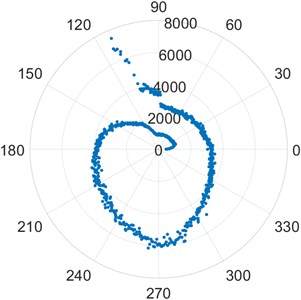
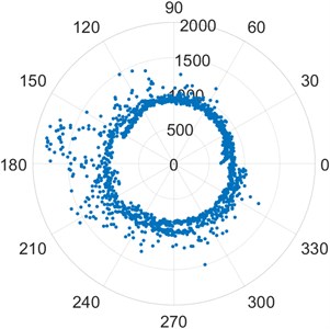
Fig. 1 denotes Poincare Maps for IMS Data Packet.
According to the IMS dataset description [29] bearings IMS1_1 and IMS1_2 are healthy at the end of the experiment. The distribution of points in Fig. 1(a) and Fig. 1(b) is uniform and concentric indicating this fact. The scale of the plot of the healthy bearings is much smaller than defective bearings. Bearing IMS1_3 has an inner race defect. The skewed distribution of points in figure Fig. 1(c) is evident due to this defect. The scale of the plot is significantly larger. There is skewing of the point distribution begins at the later stages of the experiment. Bearing IMS1_4 is known to have a spin element defect. The distinctly chaotic distribution of points along with larger than average distances from the origin in Fig. 1(d) clearly indicates the same. The plot remains roughly concentric due to the truly arbitrary distribution of points. This arbitrary distribution of points shows a spiral nature and it needs to be investigated further.
Fig. 1Poincare Maps for IMS datasets
a) [IMS1_1]
b) [IMS1_2]
c) [IMS1_3]
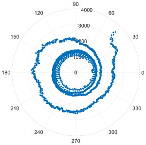
d) [IMS1_4]
e) [IMS2_1]
f) [IMS3_3]
Bearing IMS3_3 from the 3rd dataset of the IMS data packet and IMS2_1 from the second dataset are known to have an outer race failure. The highly skewed distribution of points in image Fig. 1(e) and Fig. 1(f) points to this defect. The skewing of the points starts from an earlier stage of the experiment compared to bearing IMS1_3 which had an inner race defect. Due to this, the skewing is much more pronounced. The scale is significantly larger compared to healthy bearings and slightly larger compared to the plot of IMS1_3.
5.2. FEMTO data packet
The FEMTO dataset description does not offer any results regarding the defect identified by the end of the experiment. The nature of the defect has been deduced based on IMS results and the research presented by Choy, F. K. Zhou et al [6]. This investigation has been carried out only on select bearings in the FEMTO data packet due to limited data availability on some of the bearing experiments.
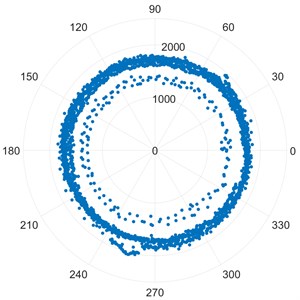
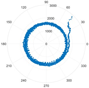
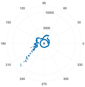
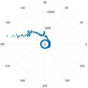
Fig. 2Poincare Maps for FEMTO datasets
a) [FEM1_2]
b) [FEM2_2]
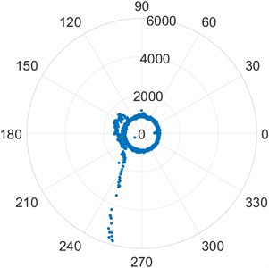
c) [FEM3_2]
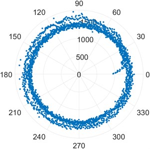
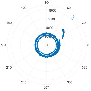
d) [FEM1_5]
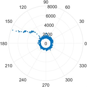
Fig. 3Poincare Maps for FEMTO datasets contd.
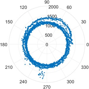
a) [FEM1_6]
b) [FEM2_3]
Poincare plots of bearings FEM1_2, FEM2_2 and FEM3_2 in the images Fig. 2(a), Fig. 2(b) and Fig. 2(c) show the skewed distribution of points characteristic of an outer race defect. The points have a skewed distribution from an early stage. The scale is much larger than that of a standard healthy bearing. Poincare plots of the bearings FEM1_5, FEM 1_6, and FEM2_3 in the images Fig. 2(d), Fig. 2(e) and Fig. 2(f) show the chaotic distribution of points and presence of outliers in terms of distance from the origin which are characteristic of a roller element defect [25]. These conclusions are drawn based on the knowledge of Poincare Maps drawn in Fig. 1 and known faults described by the experiment.
For each shaft revolution vibration signature, the Modified Poincare Map generates a representative point. Using the available shaft speed information, the Modified Poincare Map produces a point for each position of the shaft from 0 to 360. We can then create a series of Poincare Maps for each shaft position and use them to create a modified Poincare Map for shaft rotational speed. As a result, the approximate position of the defect relative to the shaft reference is determined by the start of the skewing of the points on a modified Poincare Map, while the extent of the skewing of the point distribution is an approximate measure of the defect severity. A prime example of this is Fig. 2(a) FEM1_2. It is clearly visible that the fault occurs at approximately 120 in the counterclockwise direction from the reference mark on the outer race of the bearing. The relative severity can be judged by the scale of the plot. Similarly, Fig. 2(b) shows an outer race defect approximately at the 110 mark from the reference in the counterclockwise direction. Fig. 2(c) shows an outer race defect approximately at the 140 mark from the reference point. The relative severity can be judged by the scale of the plots. The inner race defect of bearing IMS1_3 in Fig. 1(c) can be studied in a similar fashion. The defect is seen approximately at the 30 mark from the reference point. The location of spin element defects cannot be determined due to the chaotic nature of the vibration signature. The points appear arbitrary without a particular direction of skewing. Their truly arbitrary nature keeps the plot relatively concentric with a large number of outliers.
6. Fast Fourier transform results
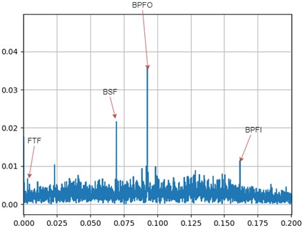
Each bearing has a unique vibration signature during its life. There are four major frequencies to take note of when analysing any bearing over an extended period of time. The Ball Spin Frequency (BSF), Fundamental Train Frequency (FTF), and Ball Pass Frequency for the Inner race (BPFI) and Ball Pass Frequency for the Outer race (BPFO).
For analysing the frequency spectrum of the bearing, a Fast Fourier Transform is used. It is to be taken note of that even though the dataset descriptions state that the bearings have only one defect, it can be seen from the following results that these bearings might have failed due to one or more defects. Multiple peaks can be seen in the graph. The ones we are concentrating on are FTF, BSF, BPFO and BPFI. But we can see that there are peaks at the multiples of these frequencies as well.
For predicting the fault in the bearing, we have used the IMS Bearing dataset as information regarding the bearing is given along with the dataset. The FEMTO bearing dataset is more suitable for predicting the RUL as time data is given accurately and no bearing information is provided.
The FTF, BSF, BPFO and BPFI values as given by the manufacturer [31] are in Table 1.
Table 1Frequency values provided by manufacturer
Vibration frequency fundamental train (FTF) | 0.0072 Hz |
Vibration frequency roller spin (BSF) | 0.0559 Hz |
Vibration frequency outer ring defect (BPFO) | 0.1217 Hz |
Vibration frequency inner ring defect (BPFI) | 0.1617 Hz |
Using IMS dataset for test sets 2 and 3, we applied Fast Fourier Transform (FFT) and the following graphs (as shown in Fig. 4, Fig. 5 Fig. 6 and Fig. 7) were obtained, similar to what we see in [27].
6.1. IMS2_1
We plotted FFT of these two sets at the beginning of test and at the end of life. The FTF undergoes a change of 10.0 %, while BSF undergoes a change of 14.65 %. The most notable shift in frequency is seen in BPFO where 25.00 % increase is found, while BPFI shifts by 1.67 %.
As seen from the above graphs (Fig. 4 and Fig. 5, BPFO undergoes the maximum shift in the frequency. This matches with the Modified Poincare Map results as shown in Fig. 1(e). Thus, we can conclude that for IMS test set 2 and Bearing 1, the fault is Outer Ring/Race Defect. Hence, the bearing fault prediction and nature of faults using FFT and Modified Poincare Map matches.
Fig. 4FFT for IMS dataset – IMS2_1 (Beginning of test)
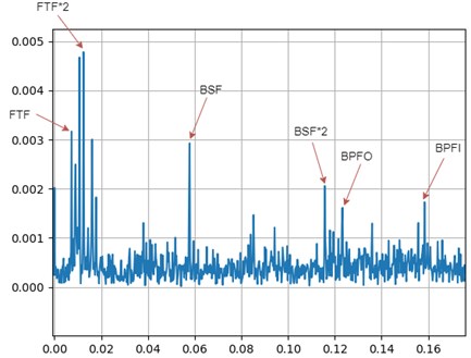
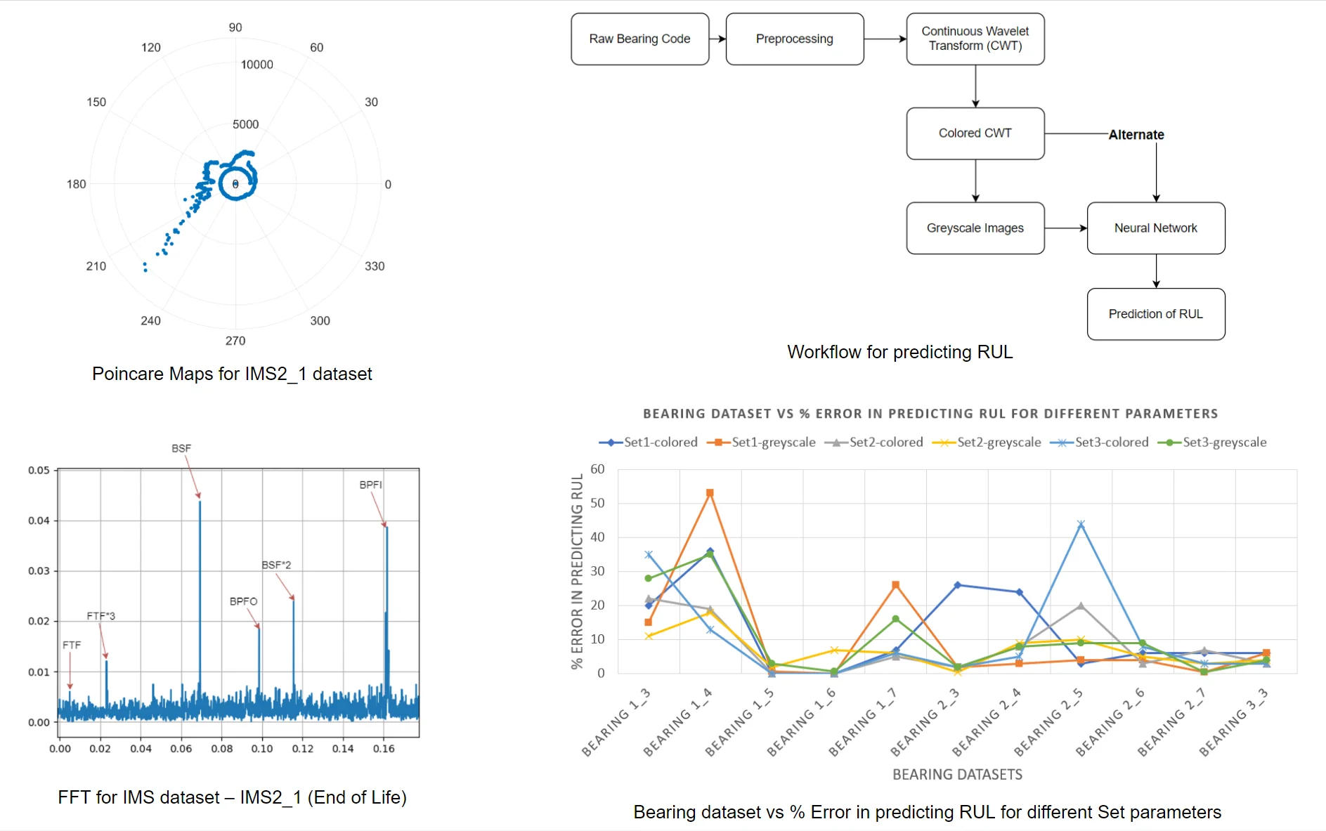
Fig. 5FFT for IMS dataset – IMS2_1 (End of Life)
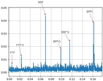
6.2. IMS3_3
The FTF undergoes a change of 2.86 %, while BSF undergoes a change of 21.05 %. The most notable shift in frequency is seen in BPFO where 36.67 % shift is found, while BPFI shifts by 3.18 %.
As seen from the above graphs (Fig. 6 and Fig. 7), BPFO undergoes the maximum shift in the frequency. This matches with the Modified Poincare Map results as shown in Fig. 1(e). Thus, we can conclude that for IMS test set 3 and Bearing 3, the fault is Outer Ring/Race Defect.
Fig. 6FFT for IMS dataset – IMS3_3 (Beginning of test)
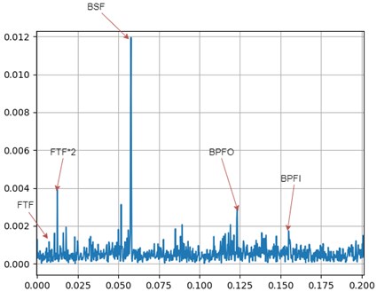
Fig. 7FFT for IMS dataset – IMS3_3 (End of Life)
7. Prediction of fraction of remaining useful life (RUL) using convolutional neural networks
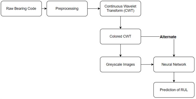
The prediction of RUL has been carried out on the FEMTO dataset since a large amount of data is available in the dataset and hence training and testing can be done properly. The path followed for predicting the fraction of remaining useful life is given in the Fig. 8.
Fig. 8Workflow for predicting RUL
7.1. Construction of CWT maps
A Continuous Wavelet Transform (CWT) is used to decompose a signal into wavelets. Wavelets are small oscillations with a high degree of temporal localization. The CWT’s basis functions are scaled and shifted versions of the time-localized mother wavelet, whereas the Fourier Transform decomposes a signal into infinite length sines and cosines, effectively losing all time-localization information. The CWT is used to create a signal’s time-frequency representation, which provides excellent time and frequency localization.
The CWT is an excellent tool for mapping non-stationary signals’ changing properties. The CWT is also an excellent technique for evaluating whether or not a signal is globally stationary. When a signal is assessed to be non-stationary, the CWT can be used to identify stationary sections of the dataset.
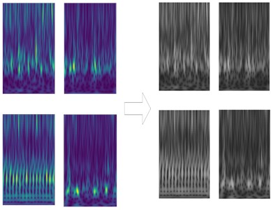
While we can use colored CWT maps to feed into the Neural network, using greyscale maps or images are proven to increase the accuracy of the model. So, we converted the colored CWT images to greyscale images using OpenCV python module [32] and obtained the result that we see in Fig. 9.
Fig. 9Conversion of colored CWT maps to greyscale CWT maps
7.2. Network construction
The effect of the network model is directly influenced by the structure of the convolutional network layer. As a result, picking the right network structure parameters is crucial.
Fig. 10Network construction
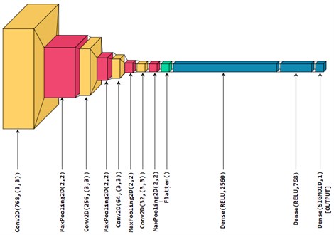
The network structure of CNN, as shown in Fig. 10, is composed of 1 input layer, 4 convolutional layers, 4 pooling layers, 2 ReLU activation layers, 1 Sigmoid activation layer (it is also the output dense layer). The size of the CWT map which was inputted via the input layer is 48×64. The sizes of the convolution kernels of the convolutional layers are all 3×3. The pooling layers are 2×2 in size. The Sigmoid and ReLU are chosen as the activation functions. Optimizer used is “Adam” and the loss function is “Mean Squared Error”. The entire CNN model was constructed using the Tensorflow [33] and Keras [34] libraries in python.
We used different convolution layer filters and tried to reach the optimum. In the graphs obtained in the Result Analysis section below, we have compared the accuracy of different convolution layer filters and activation layer density sets. Three sets are used for comparison (Table 2).
Table 2Different Sets of network parameters for CNN
Set1 | Set2 | Set3 | |
Convolution layer filters | 768, 256, 64, 32 | 1024, 512, 128, 64, 32 | 512, 256, 64, 32 |
Activation layer densities | 2560, 768, 1 | 2560, 768, 1 | 2560, 768, 300, 100, 50, 1 |
The best result was obtained with Set 2 parameters and greyscale CWT images and we have used these network parameters to obtain the best model for our CNN.
7.3. Result analysis
In the Neural Network Functioning a noticeable difference occurred when we used Set 2 network parameters from Table 2 compared to Set 1 and Set 3. So, using Set 2 parameters yields us the maximum accuracy of our CNN model.
These results are plotted in the Fig. 11.
Fig. 11Bearing dataset vs % Error in predicting RUL for different Set parameters
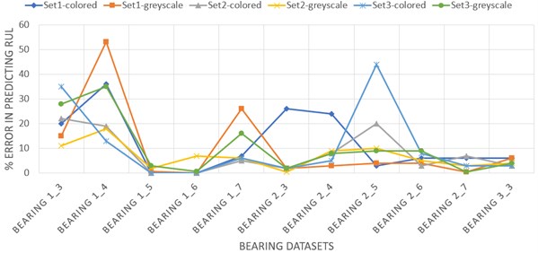
Using CWT and CNN to predict the fraction of Remaining Useful Life gave a 94.00 % median accuracy and a mean accuracy of 93.14 % on the test sets. This shows that prediction of End of Life using CNNs is a reliable technique to use when we have enough amount of data.
8. Scope of future work
Further research and experiments are required in order to use Poincare Maps to preemptively predict the fault and its location. Images of Poincare Maps generated from accelerometer data may be further used to train AI models for prediction of fault type and location. In future, different techniques like LSTM (Long short-term memory), a RNN (Recurrent Neural Network) based deep learning or a combination of CNN and LSTM can be used to increase the accuracy of the predictions. Techniques like SVM (Support Vector Machine) and Decision Trees can also be explored to check if the accuracy can be increased.
9. Conclusions
Prediction of the Bearing Faults using Modified Poincare Maps and FFT is done in this paper. Both the methods can provide us a way to detect the different types of bearing faults. Comparison of Fast Fourier Transforms (FFTs) to detect the type of bearing fault is a very simple method and doesn’t require a lot of technical expertise.
The study shows that Modified Poincare Map is a reliable method for analyzing the nonlinear vibration patterns of a roller bearing being tested until failure.
1) Non-periodic nature of the motion of spin elements cannot be detected on the frequency spectrum analysis. Poincare Maps of vibration signature arrays of large numbers of data points resolves this problem.
2) The Poincare Maps generated from the vibration accelerometer data can be reliably used to diagnose the approximate location and severity of the defect.
3) Poincare Map describes the location of the defect relatively approximately with reference to the shaft position.
4) Using CNN to predict the fraction of RUL gives a very accurate measure of the Remaining Useful Life of a bearing. In this paper, the research on RUL of the bearings was conducted using the FEMTO dataset.
5) Using CWT and CNN to predict the fraction of Remaining Useful Life gave a 94.00 % median accuracy and a mean accuracy of 93.14 % on the test sets. This shows that prediction of End of Life using CNNs is a reliable technique to use when we have enough amount of data.
6) The methodology of using CWT and CNN can also estimate the life of the bearing at any time in the entire cycle from normal operation to failure.
References
-
F. K. Choy, J. Zhou, M. J. Braun, and L. Wang, “Vibration monitoring and damage quantification of faulty ball bearings,” Journal of Tribology, Vol. 127, No. 4, pp. 776–783, Oct. 2005, https://doi.org/10.1115/1.2033899
-
R. Yuan, Y. Lv, and G. Song, “Fault diagnosis of rolling bearing based on a novel adaptive high-order local projection denoising method,” Complexity, Vol. 2018, pp. 1–15, Oct. 2018, https://doi.org/10.1155/2018/3049318
-
J. Rafiee and P. W. Tse, “Use of autocorrelation of wavelet coefficients for fault diagnosis,” Mechanical Systems and Signal Processing, Vol. 23, No. 5, pp. 1554–1572, Jul. 2009, https://doi.org/10.1016/j.ymssp.2009.02.008
-
“STM D6595-17. Test method for determination of wear metals and contaminants in used lubricating oils or used hydraulic fluids by rotating disc electrode atomic emission spectrometry,” ASTM International, West Conshohocken, PA, 2017.
-
N. J. Walker, A. N. Nowicki, “Infrared thermography handbooks,” Northampton U.K., British Institute of Non-Destructive Testing on behalf of its Condition Monitory Group, 2004.
-
Shuang Zhou, M. Xiao, Petr Bartos, M. Filip, and G. Geng, “Remaining useful life prediction and fault diagnosis of rolling bearings based on short-time Fourier transform and convolutional neural network,” Shock and Vibration, 2020.
-
S. S. Kumar, N. Mohan, P. Poornachandran, and K. P. Soman, “Condition monitoring in roller bearings using cyclostationary features,” in the Third International Symposium, pp. 690–697, 2015, https://doi.org/10.1145/2791405.2791546
-
G. Georgoulas and G. Nikolakopoulos, “Bearing fault detection and diagnosis by fusing vibration data,” in IECON Proceedings (Industrial Electronics Conference), 2016.
-
T. Han and D. Jiang, “Rolling bearing fault diagnostic method based on VMD-AR model and random forest classifier,” Shock and Vibration, Vol. 2016, pp. 1–11, 2016, https://doi.org/10.1155/2016/5132046
-
S. E. Pandarakone, Y. Mizuno, and H. Nakamura, “Algorithm and artificial intelligence neural network,” Energies, Vol. 12, 2019.
-
R. Semil and P. Jaiswal, “Bearing fault diagnosis using support vector machine with genetic algorithms based optimization and K fold cross-validation method.,” International Journal of Recent Technology and Engineering, Vol. 8, No. 2, pp. 3242–3250, Jul. 2019, https://doi.org/10.35940/ijrte.b2828.078219
-
H. O. A. Ahmed, M. L. D. Wong, and A. K. Nandi, “Intelligent condition monitoring method for bearing faults from highly compressed measurements using sparse over-complete features,” Mechanical Systems and Signal Processing, Vol. 99, pp. 459–477, Jan. 2018, https://doi.org/10.1016/j.ymssp.2017.06.027
-
A. González-Muñiz, I. Díaz, and A. A. Cuadrado, “DCNN for condition monitoring and fault detection in rotating machines and its contribution to the understanding of machine nature,” Heliyon, Vol. 6, No. 2, p. e03395, Feb. 2020, https://doi.org/10.1016/j.heliyon.2020.e03395
-
K. Worden, C. R. Farrar, J. Haywood, and M. Todd, “A review of nonlinear dynamics applications to structural health monitoring,” Structural Control and Health Monitoring, Vol. 15, No. 4, pp. 540–567, Jun. 2008, https://doi.org/10.1002/stc.215
-
F. K. Choy, S. Huangt, J. Zakrajsekt, R. F. Handschuh, and D. P. Townsendu, “Gear transmission system,” Journal of Propulsion and Power, Vol. 12, No. 2, pp. 289–295, 1996.
-
P. D. Mcfadden, “Detecting fatigue cracks in gears by amplitude and phase demodulation of the meshing vibration,” Journal of Vibration and Acoustics, Vol. 108, No. 2, pp. 165–170, Apr. 1986, https://doi.org/10.1115/1.3269317
-
B. D. Forrester, “Analysis of gear vibration in the time frequency domain,” in Proc. Of the 44th Meeting of the Mechanical Failure Prevention Group, 1990.
-
V. Polyshchuk, “Detection and quantification of the gear tooth damage from the vibration and acoustic signatures,” Ph.D. thesis, The University of Akron, Akron, 1999.
-
F. Choy, L. Wang, Jianyou Zhou, and M. Braun, “Online vibration monitoring of ball bearing damage using an experimental test rig,” Journal of Propulsion and Power, Vol. 23, No. 3, pp. 629–636, 2007.
-
Y. S. Lee, A. F. Vakakis, D. M. Mcfarland, and L. A. Bergman, “A global-local approach to nonlinear system identification: A review,” Structural Control and Health Monitoring, Vol. 17, No. 7, pp. 742–760, Nov. 2010, https://doi.org/10.1002/stc.414
-
F. C. Moon, Chaotic Vibrations. New York: John Wiley & Sons, 1987.
-
R. Brockett, “On conditions leading to chaos in feedback systems,” in 1982 21st IEEE Conference on Decision and Control, Vol. 2, No. 1, pp. 932–936, Dec. 1982, https://doi.org/10.1109/cdc.1982.268281
-
C. Bryant, P., and Jeffries, “Experimental study of driven nonlinear oscillator exhibiting hopf bifurcations, strong resonances, homoclinic bifurcations and chaotic behavior,” Lawerence Berkeley Laboratory report, LBL-16949, Technical report, 1984.
-
M. Henon, “On the numerical computation of Poincaré maps,” Physica D: Nonlinear Phenomena, Vol. 5, No. 2-3, pp. 412–414, Sep. 1982, https://doi.org/10.1016/0167-2789(82)90034-3
-
P. Singru, V. Krishnakumar, D. Natarajan, and A. Raizada, “Bearing failure prediction using Wigner-Ville distribution, modified Poincare mapping and fast Fourier transform,” Journal of Vibroengineering, Vol. 20, No. 1, pp. 127–137, Feb. 2018, https://doi.org/10.21595/jve.2017.17768
-
R. B. Randall, Vibration-based Condition Monitoring. John Wiley & Sons, 2011.
-
Y. Li, X. Liang, Y. Chen, Z. Chen, and J. Lin, “Wheelset bearing fault detection using morphological signal and image analysis,” Structural Control and Health Monitoring, Vol. 27, No. 11, pp. 1–15, Nov. 2020, https://doi.org/10.1002/stc.2619
-
D. Zhao, L. Gelman, F. Chu, and A. Ball, “Vibration health monitoring of rolling bearings under variable speed conditions by novel demodulation technique,” Structural Control and Health Monitoring, Vol. 28, No. 2, pp. 14–16, Feb. 2021, https://doi.org/10.1002/stc.2672
-
H. Qiu, J. Lee, J. Lin, and G. Yu, “Wavelet filter-based weak signature detection method and its application on rolling element bearing prognostics,” Journal of Sound and Vibration, Vol. 289, No. 4-5, pp. 1066–1090, Feb. 2006, https://doi.org/10.1016/j.jsv.2005.03.007
-
P. Nectoux et al., “Pronostia: An experimental platform for bearings accelerated life test,” in IEEE International Conference on Prognostics and Health Management, 2012.
-
“Rexnord ZA2115 Solid-housed Pillow Blocks Rex Spherical Roller Bearings,” Technical Specifications, 2021.
-
G. Bradski, “The OpenCV Library,” Dr. Dobb’s Journal of Software Tools, Vol. 120, pp. 122–125, 2000.
-
M. Abadi et al., Tensorflow: Large-Scale Machine Learning on Heterogeneous Systems, 2015.
-
F. Chollet et al., “Keras”, 2015, https://keras.io.
Cited by
About this article

